.
Integratie van GRASS GIS
The GRASS plugin provides access to GRASS GIS databases and functionalities (see GRASS-PROJECT in Verwijzingen naar literatuur en web). This includes visualizing GRASS raster and vector layers, digitizing vector layers, editing vector attributes, creating new vector layers and analysing GRASS 2-D and 3-D data with more than 400 GRASS modules.
In this section, we’ll introduce the plugin functionalities and give some examples of managing and working with GRASS data. The following main features are provided with the toolbar menu when you start the GRASS plugin, as described in section sec_starting_grass:
 Open mapset
 New mapset
 Close mapset
 Add GRASS vector layer
 Add GRASS raster layer
 Create new GRASS vector
 Edit GRASS vector layer
 Open GRASS tools
 Display current GRASS region
 Edit current GRASS region
De plug-in GRASS starten
To use GRASS functionalities and/or visualize GRASS vector and raster layers in
QGIS, you must select and load the GRASS plugin with the Plugin Manager.
Therefore, go to the menu Plugins ‣  Manage Plugins, select
  GRASS and click
[OK].
GRASS and click
[OK].
You can now start loading raster and vector layers from an existing GRASS LOCATION (see section sec_load_grassdata). Or, you can create a new GRASS LOCATION with QGIS (see section Maken van een nieuwe GRASS LOCATION) and import some raster and vector data (see section Importeren van gegevens in een GRASS LOCATION) for further analysis with the GRASS Toolbox (see section De Toolbox voor GRASS).
GRASS raster- en vectorlagen laden
With the GRASS plugin, you can load vector or raster layers using the appropriate button on the toolbar menu. As an example, we will use the QGIS Alaska dataset (see section Voorbeeldgegevens). It includes a small sample GRASS LOCATION with three vector layers and one raster elevation map.
- Create a new folder called grassdata, download the QGIS ‘Alaska’ dataset qgis_sample_data.zip from http://download.osgeo.org/qgis/data/ and unzip the file into grassdata.
- Start QGIS.
- If not already done in a previous QGIS session, load the GRASS plugin
clicking on Plugins ‣
Manage Plugins and activate GRASS.
The GRASS toolbar appears in the QGIS main window.
- In the GRASS toolbar, click the Open mapset icon
to bring up the MAPSET wizard.
- For Gisdbase, browse and select or enter the path to the newly created folder grassdata.
- You should now be able to select the LOCATION
 alaska and the MAPSET demo.
 - Click [OK]. Notice that some previously disabled tools in the GRASS toolbar are now enabled.
- Click on Add GRASS raster layer, choose the map name
gtopo30 and click [OK]. The elevation layer will be visualized.
- Click on Add GRASS vector layer, choose the map name
alaska and click [OK]. The Alaska boundary vector layer will be
overlayed on top of the gtopo30 map. You can now adapt the layer
properties as described in chapter Het dialoogvenster Vectoreigenschappen (e.g.,
change opacity, fill and outline color).
- Also load the other two vector layers, rivers and airports, and adapt their properties.
As you see, it is very simple to load GRASS raster and vector layers in QGIS. See the following sections for editing GRASS data and creating a new LOCATION. More sample GRASS LOCATIONs are available at the GRASS website at http://grass.osgeo.org/download/sample-data/.
Tip
GRASS–Laden van gegevens
If you have problems loading data or QGIS terminates abnormally, check to make sure you have loaded the GRASS plugin properly as described in section De plug-in GRASS starten.
GRASS LOCATION en MAPSET
GRASS data are stored in a directory referred to as GISDBASE. This directory, often called grassdata, must be created before you start working with the GRASS plugin in QGIS. Within this directory, the GRASS GIS data are organized by projects stored in subdirectories called LOCATIONs. Each LOCATION is defined by its coordinate system, map projection and geographical boundaries. Each LOCATION can have several MAPSETs (subdirectories of the LOCATION) that are used to subdivide the project into different topics or subregions, or as workspaces for individual team members (see Neteler & Mitasova 2008 in Verwijzingen naar literatuur en web). In order to analyze vector and raster layers with GRASS modules, you must import them into a GRASS LOCATION. (This is not strictly true – with the GRASS modules r.external and v.external you can create read-only links to external GDAL/OGR-supported datasets without importing them. But because this is not the usual way for beginners to work with GRASS, this functionality will not be described here.)
Figure GRASS location 1:
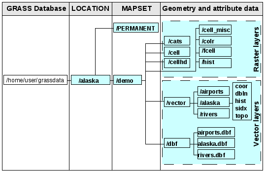
Gegevens voor GRASS op de LOCATION alaska
Maken van een nieuwe GRASS LOCATION
As an example, here is how the sample GRASS LOCATION alaska, which is projected in Albers Equal Area projection with unit feet was created for the QGIS sample dataset. This sample GRASS LOCATION alaska will be used for all examples and exercises in the following GRASS-related sections. It is useful to download and install the dataset on your computer (see Voorbeeldgegevens).
- Start QGIS and make sure the GRASS plugin is loaded.
- Visualize the alaska.shp shapefile (see section Loading a Shapefile) from the QGIS Alaska dataset (see Voorbeeldgegevens).
- In the GRASS toolbar, click on the New mapset icon
to bring up the MAPSET wizard.
Selecteer een bestaande GRASS-database (GISDBASE) map grassdata, of maak een nieuwe LOCATION met behulp van een bestandsbeheerder op uw computer. Klik dan op [Next].
- We can use this wizard to create a new MAPSET within an existing
LOCATION (see section Toevoegen van een nieuwe MAPSET) or to create a new
LOCATION altogether. Select
 Create new
location (see figure_grass_location_2).
Create new
location (see figure_grass_location_2). Voer een naam in voor de LOCATION – wij gebruikten ‘alaska’ – en klik op [Next].
- Define the projection by clicking on the radio button
Projection to enable the projection list.
- We are using Albers Equal Area Alaska (feet) projection. Since we happen to
know that it is represented by the EPSG ID 2964, we enter it in the search box.
(Note: If you want to repeat this process for another LOCATION and
projection and haven’t memorized the EPSG ID, click on the
 CRS Status icon in the lower right-hand corner of the status bar (see
section Werken met projecties)).
CRS Status icon in the lower right-hand corner of the status bar (see
section Werken met projecties)). In Filter, voer 2964 in om de projectie te selecteren.
Klik op [Next].
- To define the default region, we have to enter the LOCATION bounds in the north, south, east, and west directions. Here, we simply click on the button [Set current |qg| extent], to apply the extent of the loaded layer alaska.shp as the GRASS default region extent.
Klik op [Next].
We moeten ook een MAPSET definiëren binnen onze nieuwe LOCATION (dit is nodig bij het maken van een nieuwe LOCATION). U mag het de naam geven die u wilt - wij gebruikten ‘demo’. GRASS maakt automatisch een speciale MAPSET, genaamd PERMANENT, ontworpen om de brongegevens voor het project op te slaan, het standaard ruimtelijke bereik en de definities van het coördinatensysteem (zie Neteler & Mitasova 2008 in Verwijzingen naar literatuur en web).
Controleer de samenvatting om te zien of die juist is en klik op [Finish].
De nieuwe LOCATION, ‘alaska’, en de twee MAPSETs, ‘demo’ en ‘PERMANENT’, zijn gemaakt. De momenteel geopende werkset is ‘demo’, zoals u heeft gedefinieerd.
Merk op dat enkele gereedschappen op de werkbalk van GRASS, die uitgeschakeld waren, nu zijn ingeschakeld.
Figure GRASS location 2:
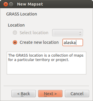
Creating a new GRASS LOCATION or a new MAPSET in QGIS
If that seemed like a lot of steps, it’s really not all that bad and a very quick way to create a LOCATION. The LOCATION ‘alaska’ is now ready for data import (see section Importeren van gegevens in een GRASS LOCATION). You can also use the already-existing vector and raster data in the sample GRASS LOCATION ‘alaska’, included in the QGIS ‘Alaska’ dataset Voorbeeldgegevens, and move on to section Het GRASS vectorgegevensmodel.
Toevoegen van een nieuwe MAPSET
A user has write access only to a GRASS MAPSET he or she created. This means that besides access to your own MAPSET, you can read maps in other users’ MAPSETs (and they can read yours), but you can modify or remove only the maps in your own MAPSET.
Alle MAPSET's bevatten een bestand WIND dat de huidige waarden voor coördinaten voor de grenzen opslaat en de huidige geselecteerd rasterresolutie (zie Neteler & Mitasova 2008 in Verwijzingen naar literatuur en web, en het gedeelte Het GRASS–gereedschap regio).
- Start QGIS and make sure the GRASS plugin is loaded.
- In the GRASS toolbar, click on the New mapset icon
to bring up the MAPSET wizard.
Selecteer de GRASS database (GISDBASE)-map grassdata met de LOCATION ‘alaska’, waar we nog een MAPSET zullen toevoegen, genaamd ‘test’.
Klik op [Next].
- We can use this wizard to create a new MAPSET within an existing
LOCATION or to create a new LOCATION altogether. Click on the
radio button Select location
(see figure_grass_location_2) and click [Next].
Voer de naam text in voor de nieuwe MAPSET. Onder in de assistent ziet u een lijst van bestaande MAPSET's en corresponderende eigenaren.
Klik op [Next], controleer de samenvatting om te zien of die juist is en klik op [Finish].
Importeren van gegevens in een GRASS LOCATION
This section gives an example of how to import raster and vector data into the ‘alaska’ GRASS LOCATION provided by the QGIS ‘Alaska’ dataset. Therefore, we use the landcover raster map landcover.img and the vector GML file lakes.gml from the QGIS ‘Alaska’ dataset (see Voorbeeldgegevens).
- Start QGIS and make sure the GRASS plugin is loaded.
- In the GRASS toolbar, click the Open MAPSET icon
to bring up the MAPSET wizard.
- Select as GRASS database the folder grassdata in the QGIS Alaska dataset, as LOCATION ‘alaska’, as MAPSET ‘demo’ and click [OK].
- Now click the Open GRASS tools icon. The
GRASS Toolbox (see section De Toolbox voor GRASS) dialog appears.
Klik op de module r.in.gdal op de tab Modulen Boom om de rasterkaart landcover.img te importeren. Deze module voor GRASS stelt u in staat GDAL-ondersteunde rasterbestanden te importeren in een LOCATION van GRASS. Het dialoogvenster voor de module r.in.gdal verschijnt.
- Browse to the folder raster in the QGIS ‘Alaska’ dataset and select the file landcover.img.
Definieer, als naam voor het raster-uitvoerbestand, landcover_grass en klik op [Uitvoeren]. Op de tab Output ziet u de momenteel uitgevoerde opdracht voor GRASS r.in.gdal -o input=/pad/naar/landcover.img output=landcover_grass.
- When it says Succesfully finished, click [View output]. The landcover_grass raster layer is now imported into GRASS and will be visualized in the QGIS canvas.
Klik op de module v.in.ogr op de tab Modulen Boom om het vector GML-bestand lakes.gml te importeren. Deze module voor GRASS stelt u in staat OGR-ondersteunde vectorbestanden te importeren in een LOCATION van GRASS. Het dialoogvenster voor de module v.in.ogr verschijnt.
- Browse to the folder gml in the QGIS ‘Alaska’ dataset and select the file lakes.gml as OGR file.
Definieer, als naam voor het vector-uitvoerbestand, lakes_grass en klik op [Uitvoeren]. U hoeft zich in dit voorbeeld geen zorgen te maken over de andere opties. Op de tab Output ziet u de momenteel uitgevoerde opdracht van GRASS v.in.ogr -o dsn=/pad/naar/lakes.gml output=lakes\_grass.
- When it says Succesfully finished, click [View output]. The lakes_grass vector layer is now imported into GRASS and will be visualized in the QGIS canvas.
Het GRASS vectorgegevensmodel
It is important to understand the GRASS vector data model prior to digitizing.
In general, GRASS uses a topological vector model.
This means that areas are not represented as closed polygons, but by one or more boundaries. A boundary between two adjacent areas is digitized only once, and it is shared by both areas. Boundaries must be connected and closed without gaps. An area is identified (and labeled) by the centroid of the area.
Naast grenzen en zwaartepunten kan een vectorkaart ook punten en lijnen bevatten. Al deze elementen voor geometrie kunnen worden gemixt in één vector en zullen worden weergegeven in verschillende, zogenaamde ‘lagen’, binnen één vectorkaart van GRASS. Dus in GRASS, is een laag geen vector- of rasterkaart, maar een niveau binnen een vectorlaag. Het is belangrijk om dit verschil zorgvuldig te onderscheiden. (Hoewel het mogelijk is om elementen voor geometrie te mixen, het is ongebruikelijk en, zelfs in GRASS, alleen gebruikt in speciale gevallen, zoals vector netwerkanalyses. Normaal gesproken zou u de voorkeur hebben voor het opslaan van verschillende elementen voor geometrie in verschillende lagen.)
Het is mogelijk om verscheidene ‘lagen’ op te slaan in één vector-gegevensset. Bijvoorbeeld: velden, bossen en meren kunnen worden opgeslagen in één vector. Een aansluitend bos en meer kunnen dezelfde grens delen, maar zij hebben afzonderlijk attributentabellen. Het is ook mogelijk attributen te verbinden aan grenzen. Een voorbeeld zou kunnen zijn het geval waar de grens tussen een meer en een bos een weg is, dus kan het een verschillende attributentabel hebben.
De ‘laag’ van het object wordt gedefinieerd door de ‘laag’ binnen GRASS. ‘Laag’ is het getal dat definieert of er meer dan één laag binnen de gegevensset is (bijv., als de geometrie bos of meer is). Momenteel mag het alleen een getal zijn. In de toekomst zal GRASS ook namen als velden in de gebruikersinterface ondersteunen.
Attributes can be stored inside the GRASS LOCATION as dBase or SQLite3 or in external database tables, for example, PostgreSQL, MySQL, Oracle, etc.
Attributen in databasetabellen worden aan elementen van geometrie gekoppeld door middel van een waarde ‘categorie’.
‘Category’ (sleutel, ID) is een integer die is verbonden met geometrie-primitieven, en het wordt gebruikt als de koppeling naar één sleutelkolom in de databasetabel.
Tip
Het GRASS vectorgegevensmodel leren
De beste manier om het vectormodel van GRASS en de mogelijkheden daarvan is om één van de vele handleidingen voor GRASS te downloaden waar het vectormodel dieper wordt beschreven. Zie http://grass.osgeo.org/documentation/manuals/ voor meer informatie, boeken en handleidingen in verschillende talen.
Maken van een nieuwe GRASS vectorlaag
To create a new GRASS vector layer with the GRASS plugin, click the
Create new GRASS vector toolbar icon.
Enter a name in the text box, and you can start digitizing point, line or polygon
geometries following the procedure described in section Digitaliseren en bewerken van een GRASS vectorlaag.
In GRASS, it is possible to organize all sorts of geometry types (point, line and area) in one layer, because GRASS uses a topological vector model, so you don’t need to select the geometry type when creating a new GRASS vector. This is different from shapefile creation with QGIS, because shapefiles use the Simple Feature vector model (see section Nieuwe vectorlagen maken).
Tip
Creating an attribute table for a new GRASS vector layer
If you want to assign attributes to your digitized geometry features, make sure to create an attribute table with columns before you start digitizing (see figure_grass_digitizing_5).
Digitaliseren en bewerken van een GRASS vectorlaag
The digitizing tools for GRASS vector layers are accessed using the
Edit GRASS vector layer icon on the toolbar. Make sure you
have loaded a GRASS vector and it is the selected layer in the legend before
clicking on the edit tool. Figure figure_grass_digitizing_2 shows the GRASS
edit dialog that is displayed when you click on the edit tool. The tools and
settings are discussed in the following sections.
Tip
Digitaliseren van polygonen in GRASS
If you want to create a polygon in GRASS, you first digitize the boundary of the polygon, setting the mode to ‘No category’. Then you add a centroid (label point) into the closed boundary, setting the mode to ‘Next not used’. The reason for this is that a topological vector model links the attribute information of a polygon always to the centroid and not to the boundary.
Werkbalk
In figure_grass_digitizing_1, you see the GRASS digitizing toolbar icons provided by the GRASS plugin. Table table_grass_digitizing_1 explains the available functionalities.
Figure GRASS digitizing 1:

GRASS Digitizing Toolbar
Pictogram |
Gereedschap |
Doel |
|---|---|---|
 |
Nieuw punt |
Nieuw punt digitaliseren |
 |
Nieuwe lijn |
Nieuwe lijn digitaliseren |
 |
Nieuwe grens |
Digitize new boundary (finish by selecting new tool) |
 |
Nieuw zwaartepunt |
Nieuw zwaartepunt digitaliseren (label bestaand gebied) |
 |
Move vertex | Move one vertex of existing line or boundary and identify new position |
 |
Add vertex | Add a new vertex to existing line |
 |
Delete vertex | Delete vertex from existing line (confirm selected vertex by another click) |
 |
Move element | Move selected boundary, line, point or centroid and click on new position |
 |
Split line | Split an existing line into two parts |
 |
Delete element | Delete existing boundary, line, point or centroid (confirm selected element by another click) |
 |
Edit attributes | Edit attributes of selected element (note that one element can represent more features, see above) |
 |
Close | Close session and save current status (rebuilds topology afterwards) |
Tabel GRASS Digitaliseren 1: GRASS Gereedschap Digitaliseren
Category Tab
The Category tab allows you to define the way in which the category values will be assigned to a new geometry element.
Figure GRASS digitizing 2:
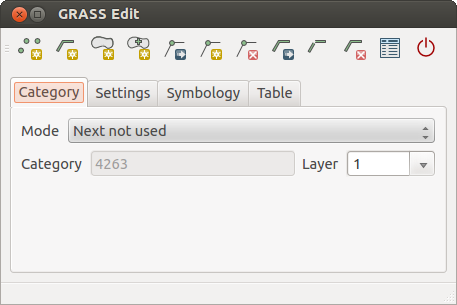
GRASS Digitizing Category Tab
- Mode: The category value that will be applied to new geometry elements.
- Next not used - Apply next not yet used category value to geometry element.
- Manual entry - Manually define the category value for the geometry element in the ‘Category’ entry field.
- No category - Do not apply a category value to the geometry element. This is used, for instance, for area boundaries, because the category values are connected via the centroid.
- Category - The number (ID) that is attached to each digitized geometry element. It is used to connect each geometry element with its attributes.
- Field (layer) - Each geometry element can be connected with several attribute tables using different GRASS geometry layers. The default layer number is 1.
Tip
Creating an additional GRASS ‘layer’ with |qg|
If you would like to add more layers to your dataset, just add a new number in the ‘Field (layer)’ entry box and press return. In the Table tab, you can create your new table connected to your new layer.
Settings Tab
The Settings tab allows you to set the snapping in screen pixels. The threshold defines at what distance new points or line ends are snapped to existing nodes. This helps to prevent gaps or dangles between boundaries. The default is set to 10 pixels.
Figure GRASS digitizing 3:
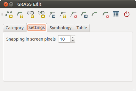
GRASS Digitizing Settings Tab
Symbology Tab
The Symbology tab allows you to view and set symbology and color settings for various geometry types and their topological status (e.g., closed / opened boundary).
Figure GRASS digitizing 4:
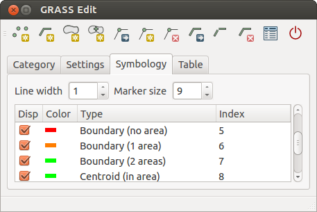
GRASS Digitizing Symbology Tab
Table Tab
The Table tab provides information about the database table for a given ‘layer’. Here, you can add new columns to an existing attribute table, or create a new database table for a new GRASS vector layer (see section Maken van een nieuwe GRASS vectorlaag).
Figure GRASS digitizing 5:
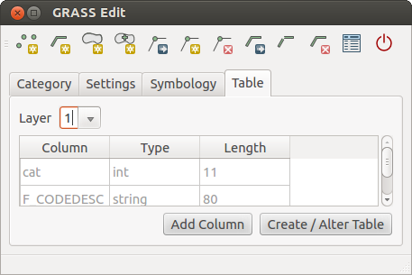
GRASS Digitizing Table Tab
Tip
GRASS Rechten voor bewerken
U moet de eigenaar zijn van de MAPSET van GRASS die u wilt bewerken. Het is onmogelijk om gegevenslagen te bewerken in een MAPSET die niet van u is, zelfs niet als u schrijfrechten heeft.
Het GRASS–gereedschap regio
De definitie van een regio (instellen van een ruimtelijk werkvenster) in GRASS is belangrijk voor het werken met rasterlagen. Vectoranalyses zijn standaard niet beperkt tot definities van gedefinieerde regio´s. Maar alle nieuwe gemaakte rasters zullen de ruimtelijke extensie en resolutie van de huidige gedefinieerde regio in GRASS hebben, ongeacht hun originele extensie en resolutie. De huidige regio van GRASS is opgeslagen in het bestand $LOCATION/$MAPSET/WIND, en het definieert de grenzen voor Noord, Zuid, Oost en West, aantal kolommen en rijen, horizontale en verticale ruimtelijke resolutie.
It is possible to switch on and off the visualization of the GRASS region in the QGIS
canvas using the Display current GRASS region button.
With the Edit current GRASS region icon, you can open
a dialog to change the current region and the symbology of the GRASS region
rectangle in the QGIS canvas. Type in the new region bounds and resolution, and
click [OK]. The dialog also allows you to select a new region interactively with your
mouse on the QGIS canvas. Therefore, click with the left mouse button in the QGIS
canvas, open a rectangle, close it using the left mouse button again and click
[OK].
De module voor GRASS g.region verschaft nog veel meer parameters om een toepasselijk bereik voor een regio en resolutie voor uw rasteranalyses te definiëren. U kunt deze parameters gebruiken met de Toolbox voor GRASS, beschreven in het gedeelte De Toolbox voor GRASS.
De Toolbox voor GRASS
The Open GRASS Tools box provides GRASS module functionalities
to work with data inside a selected GRASS LOCATION and MAPSET.
To use the GRASS Toolbox you need to open a LOCATION and MAPSET
that you have write permission for (usually granted, if you created the MAPSET).
This is necessary, because new raster or vector layers created during analysis
need to be written to the currently selected LOCATION and MAPSET.
Figure GRASS Toolbox 1:
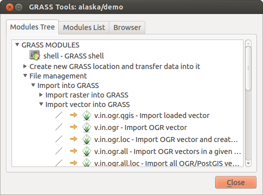
GRASS Toolbox en Moduleboom 
Werken met modules van GRASS
De GRASS-shell binnen de Toolbox voor GRASS verschaft toegang tot bijna alle (meer dan 300) modules voor GRASS in een interface voor de opdrachtregel. Ongeveer 200 van de beschikbare modules en functionaliteiten voor GRASS zijn ook voorzien van grafische dialoogvensters binnen de Toolbox van de plug-in GRASS om een meer gebruikersvriendelijker werkomgeving te bieden.
A complete list of GRASS modules available in the graphical Toolbox in QGIS version 2.8 is available in the GRASS wiki at http://grass.osgeo.org/wiki/GRASS-QGIS_relevant_module_list.
Het is ook mogelijk de inhoud van de Toolbox van GRASS aan te passen. Deze procedure wordt beschreven in het gedeelte Aanpassen van de Toolbox van GRASS.
Zoals weergegeven in figure_grass_toolbox_1 kunt u naar de toepasselijke module voor GRASS zoeken met behulp van de thematisch gegroepeerde Modulen Boom of de te doorzoeken tab Modulen Lijst.
Door te klikken op een grafisch pictogram voor een module zal een nieuwe tab worden toegevoegd aan het dialoogvenster van de Toolbox, die drie nieuwe sub-tabs verschaft: Opties, Output en Handleiding.
Opties
The Options tab provides a simplified module dialog where you can usually select a raster or vector layer visualized in the QGIS canvas and enter further module-specific parameters to run the module.
Figure GRASS module 1:
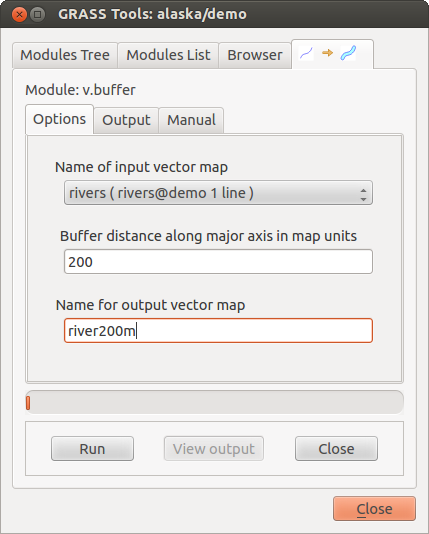
GRASS Toolbox Module-opties
The provided module parameters are often not complete to keep the dialog clear. If you want to use further module parameters and flags, you need to start the GRASS shell and run the module in the command line.
A new feature since QGIS 1.8 is the support for a Show Advanced Options button below the simplified module dialog in the Options tab. At the moment, it is only added to the module v.in.ascii as an example of use, but it will probably be part of more or all modules in the GRASS Toolbox in future versions of QGIS. This allows you to use the complete GRASS module options without the need to switch to the GRASS shell.
Output
Figure GRASS module 2:
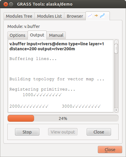
GRASS Toolbox Module Output
De tab Output verschaft informatie over de uitvoerstatus van de module. Wanneer u klikt op de knop [Uitvoeren], schakelt de module naar de tab Output en ziet u informatie over het analyseproces. Als alles goed werkt ziet u uiteindelijk een bericht Succesvol geëindigd.
Handleiding
Figure GRASS module 3:
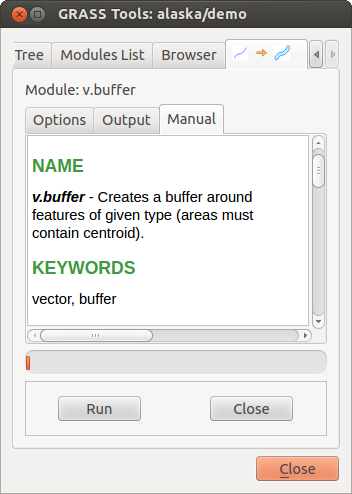
GRASS Toolbox Module Handleiding
De tab Handleiding geeft de HTML Help-pagina van de module voor GRASS weer. U kunt die gebruiken om te controleren op meer parameters en vlaggen voor de module of om een beter inzicht te krijgen over het doel van de module. Aan het einde van elke pagina met de handleiding van de module zult u verder koppelingen zien naar de Main index, de Thematische index en de Full index. Deze koppelingen verschaffen dezelfde informatie als de module g.manual.
Tip
Resultaten onmidellijk weergeven
Als u uw resultaten van de berekeningen direct wilt weergeven in uw kaartvenster, kunt u de knop ‘Uitvoer bekijken’ onder op de tab van de module gebruiken.
GRASS voorbeelden van modules
De volgende voorbeelden zullen de kracht van enkele van de modules van GRASS demonstreren.
Contourlijnen maken
Het eerste voorbeeld maakt een vector contourenkaart uit een hoogteraster (DEM). Hier wordt aangenomen dat u de LOCATION Alaska heeft ingesteld zoals uitgelegd in het gedeelte Importeren van gegevens in een GRASS LOCATION.
- First, open the location by clicking the
Open mapset button and choosing the Alaska location.
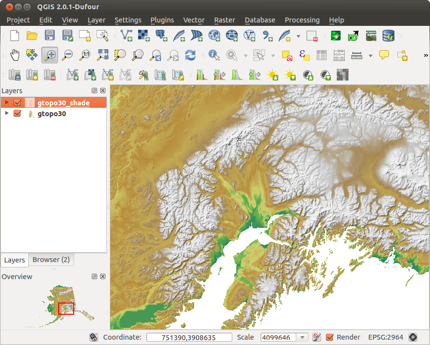
- Now load the gtopo30 elevation raster by clicking
Add GRASS raster layer and selecting the
gtopo30 raster from the demo location.
- Now open the Toolbox with the Open GRASS tools button.
In de lijst met categorieën gereedschap, dubbelklik op Raster ‣ ‘Surface management’ ‣ Genereer vector contourlijnen.
- Now a single click on the tool r.contour will open the tool dialog as explained above (see Werken met modules van GRASS). The gtopo30 raster should appear as the Name of input raster.
- Type into the Increment between Contour levels
 the value 100. (This will create contour lines at intervals of 100 meters.)
 Typ in het vak Name for output vector map de naam ctour_100.
Klik op [Uitvoeren] om het proces te beginnen. Wacht even totdat het bericht Succesvol geëindigd verschijnt in het uitvoervenster. Klik dan op [Uitvoer bekijken] en [Sluiten].
Omdat dit een grote regio is zal het even duren voordat alles wordt weergegeven. Nadat het renderen is voltooid, kunt u het venster Laageigenschappen openen om de lijnkleur te wijzigen zodat de contouren duidelijk over het hoogteraster te zien zijn, zoals in Het dialoogvenster Vectoreigenschappen.
Zoom vervolgens in op een klein bergachtig gebied in het midden van Alaska. Bij het veel inzoomen zult u opmerken dat de contouren scherpe hoeken hebben. GRASS biedt het gereedschap v.generalize om vectorkaarten lichtjes te wijzigen met behoud van hun overall-vorm. Het gereedschap gebruikt verscheidene verschillende algoritmen met verschillende doeleinden. Sommig algoritmen (d.i., Douglas Peuker en Vertex Reduction) vereenvoudigen de lijn door enkele punten te verwijderen. De resulterende vector zal sneller laden. Dit proces is nuttig als u een vector met veel detail heeft, maar u maakt een kaart op zeer kleine schaal, dus detail is niet nodig.
Tip
Het gereedschap Vereenvoudigen
Note that the QGIS fTools plugin has a Simplify geometries ‣ tool that works just like the GRASS v.generalize Douglas-Peuker algorithm.
Echter, het doel van dit voorbeeld is anders. De contourlijnen die zijn gemaakt door r.contour hebben scherpe hoeken die gladder zouden moeten. Tussen de algoritmen voor v.generalize staat Chaiken’s, wat precies dat doet (ook Hermite-splines). Onthoud dat deze algoritmen aanvullende hoeken kunnen toevoegen aan de vector, waardoor het nog langzamer is te laden.
Open de Toolbox voor GRASS en dubbelklik op categorieën Vector ‣ Develop map ‣ Generaliseren, klik dan op de module v.generalize om het venster Opties daarvan te openen.
Controleer of de vectorlaag ‘ctour_100’ verschijnt in het vak Name of input vector.
Kies Chaiken’s Algorithm uit de lijst met algoritmen. Laat alle andere opties op hun standaard staan en scroll naar beneden naar de laatste rij om in het veld Name for output vector map ‘ctour_100_smooth’ in te vullen en klik op [Uitvoeren].
Het proces duurt enige tijd. Als eenmaal Succesvol geëindigd verschijnt in het uitvoervenster, klik dan op [Uitvoer bekijken] en dan op [Sluiten].
U zou de kleur van de vectorlaag kunnen wijzigen om die duidelijk weer te geven tegen de achtergrond van het raster en om contrast te krijgen met de originele contourlijnen. Het zal u opvallen dat de nieuwe contourlijnen gladdere hoeken hebben dan de originele terwijl zij nog voldoen aan de originele overall-vorm.
Figure GRASS module 4:
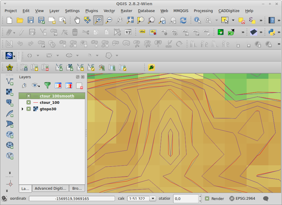
GRASS module v.generalize om een vectorkaart gladder te maken
Tip
Ander gebruik voor r.contour
De hierboven beschreven procedure kan in equivalente andere situaties worden gebruikt. Als u een rasterkaart heeft met gegevens over neerslag, bijvoorbeeld, dan kan dezelfde methode worden gebruikt om een vectorkaart met isohyetale (constante neerslag) lijnen te maken.
Een 3D heuvels met schaduw-effect maken
Verscheidene methoden worden gebruikt om hoogtelagen weer te geven en een 3D-effect aan kaarten te geven. Het gebruiken van contourlijnen, zoals hierboven weergegeven, is een populaire methode die vaak gekozen wordt om topografische kaarten te produceren. Een andere manier om een 3D-effect weer te geven is door schaduw op heuvels. Het effect van schaduw op heuvels wordt gemaakt vanuit een DEM (hoogte)raster door eerst de helling en aspect van elke cel te berekenen, dan de positie van de zon in de lucht te simuleren en een waarde van reflectie te geven aan elke cel. U krijgt dus lichte hellingen in de zon; de hellingen die uit de zon liggen (in de schaduw) worden donkerder.
Begin dit voorbeeld met het laden van het hoogteraster gtopo30. Start de Toolbox voor GRASS en onder de categorie Raster, dubbelklik om Ruimtelijke analyse ‣ Terrain analysis te openen.
Klik dan op r.shaded.relief om de module te openen.
- Change the azimuth angle 270 to 315.
Voer gtopo30_shade in voor het nieuwe raster met schaduw voor de heuvels en klik op [Uitvoeren].
Wanneer het proces voltooid is, voeg dan het raster met schaduw voor de heuvels toe aan de kaart. U zou die nu moeten zien weergegeven in grijswaarden.
Verplaats de kaart met schaduw op de heuvels naar onder de kaart gtopo30 in de inhoudsopgave, open dan het venster Properties van gtopo30, schakel naar de tab Transparantie en stel het niveau voor transparantie in op ongeveer 25% om zowel de schaduw op de heuvels als de kleuren van gtopo30 tezamen te zien.
U zou nu de hoogte gtopo30 moeten hebben met zijn kleurenkaart en transparante instelling weergegeven boven de kaart van de heuvels met schaduw in grijswaarden. Schakel, om de visuele effecten van de schaduw op de hevels te zien, de kaart gtopo30_shade uit en schakel die dan weer in.
Gebruiken van de GRASS-shell
The GRASS plugin in QGIS is designed for users who are new to GRASS and not familiar with all the modules and options. As such, some modules in the Toolbox do not show all the options available, and some modules do not appear at all. The GRASS shell (or console) gives the user access to those additional GRASS modules that do not appear in the Toolbox tree, and also to some additional options to the modules that are in the Toolbox with the simplest default parameters. This example demonstrates the use of an additional option in the r.shaded.relief module that was shown above.
Figure GRASS module 5:
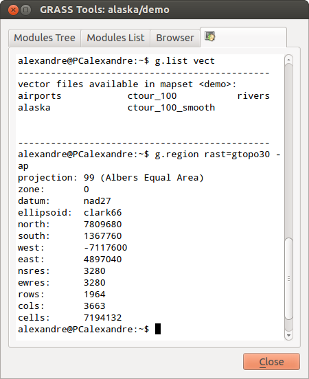
De GRASS-shell, r.shaded.relief module
De module r.shaded.relief mag een parameter zmult hebben, die de waarden voor hoogte relatief vermenigvuldigt ten opzichte van de eenheden van de XY-coördinaten zodat het effect van schaduw op de heuvels nog meer geprononceerd is.
Laad het hoogteraster gtopo30 zoals hierboven en start dan de Toolbox voor GRASS en klik op de GRASS-shell. Type, in het venster van de shell, de opdracht r.shaded.relief map=gtopo30 shade=gtopo30_shade2 azimuth=315 zmult=3 en druk op [Enter].
- After the process finishes, shift to the Browse tab and double-click on the new gtopo30_shade2 raster to display it in QGIS.
Zoals hierboven uitgelegd, verplaats het raster met het schaduw-reliëf tot onder het raster gtopo30 in de inhoudsopgave en controleer de transparantie van de gekleurde laag gtopo30. U zou moeten zien dat het 3D-effect sterker naar voren komt vergeleken met de eerste kaart met schaduw-reliëf.
Figure GRASS module 6:
Weergeven van reliëf met schaduw, gemaakt met de module van GRASS r.shaded.relief
Rasterstatistieken in een vectorkaart
Het volgende voorbeeld laat zien hoe een module van GRASS rastergegevens kan aggregeren en kolommen voor statistieken voor elke polygoon in een vectorkaart kan toevoegen.
Gebruik opnieuw de gegevens voor Alaska, bekijk Importeren van gegevens in een GRASS LOCATION om het shapefile trees te importeren vanuit de map shapefiles in GRASS.
Nu is een tussenstap vereist: zwaartepunten moeten worden toegevoegd aan de geïmporteerde kaart trees om het een volledige gebiedsvector voor GRASS te maken (inclusief beide grenzen en zwaartepunten).
Kies, vanuit de Toolbox, Vectorlaag ‣ Develop map ‣ Objecten beheren en open de module v.centroids.
Voer als output vector map in ‘forest_areas’ en voer de module uit.
- Now load the forest_areas vector and display the types of forests - deciduous,
evergreen, mixed - in different colors: In the layer Properties
window, Symbology tab, choose from Legend type
‘Unique value’ and set the Classification field
to ‘VEGDESC’. (Refer to the explanation of the symbology tab in
Menu Stijl of the vector section.)
Vervolgens, open de Toolbox voor GRASS opnieuw en open Vectorlaag ‣ Vector updaten o.b.v. andere kaarten.
Klik op de module v.rast.stats. Voer gtopo30 en forest_areas in.
Er is slechts één aanvullende parameter nodig: Voer column prefix elev in en klik op [Uitvoeren]. Dit is een qua berekeningen zware bewerking die geruime tijd zal vergen (waarschijnlijk meer dan twee uur).
Tenslotte, open de attributentabel van forest_areas en verifieer dat verschillende nieuwe kolommen zijn toegevoegd, inclusief elev_min, elev_max, elev_mean, etc., voor elk polygoon bos.
Working with the GRASS LOCATION browser
Another useful feature inside the GRASS Toolbox is the GRASS LOCATION browser. In figure_grass_module_7, you can see the current working LOCATION with its MAPSETs.
In the left browser windows, you can browse through all MAPSETs inside the current LOCATION. The right browser window shows some meta-information for selected raster or vector layers (e.g., resolution, bounding box, data source, connected attribute table for vector data, and a command history).
Figure GRASS module 7:
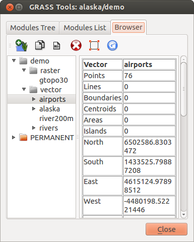
GRASS LOCATION browser
The toolbar inside the Browser tab offers the following tools to manage the selected LOCATION:
 Add selected map to canvas
 Copy selected map
 Rename selected map
 Delete selected map
 Set current region to selected map
 Refresh browser window
The Rename selected map and
Delete selected map only work with maps inside your currently selected
MAPSET. All other tools also work with raster and vector layers in
another MAPSET.
Aanpassen van de Toolbox van GRASS
Nagenoeg alle modules voor GRASS kunnen worden toegevoegd aan de Toolbox voor GRASS. Een XML-interface wordt verschaft voor het parsen van de vrij eenvoudige XML-bestanden die het uiterlijk en parameters van de module binnen de Toolbox configureren.
Een voorbeeld XML-bestand voor het maken van de module v.buffer (v.buffer.qgm) ziet er uit zoals dit:
<?xml version="1.0" encoding="UTF-8"?>
<!DOCTYPE qgisgrassmodule SYSTEM "http://mrcc.com/qgisgrassmodule.dtd">

<qgisgrassmodule label="Vector buffer" module="v.buffer">
        <option key="input" typeoption="type" layeroption="layer" />
        <option key="buffer"/>
        <option key="output" />
</qgisgrassmodule>
The parser reads this definition and creates a new tab inside the Toolbox when you select the module. A more detailed description for adding new modules, changing a module’s group, etc., can be found on the QGIS wiki at http://hub.qgis.org/projects/quantum-gis/wiki/Adding_New_Tools_to_the_GRASS_Toolbox.