Intégration du SIG GRASS¶

Lancer l’extension GRASS¶

To use GRASS functionalities and/or visualize GRASS vector and raster layers in QGIS, you must select and load the GRASS plugin with the Plugin Manager. Therefore, go to the menu Plugins ‣ Manage Plugins, select GRASS and click [OK].

You can now start loading raster and vector layers from an existing GRASS LOCATION (see section sec_load_grassdata). Or, you can create a new GRASS LOCATION with QGIS (see section Créer un nouveau SECTEUR GRASS) and import some raster and vector data (see section Importer des données dans un SECTEUR GRASS) for further analysis with the GRASS Toolbox (see section La Boîte à outils GRASS).

Charger des données GRASS raster et vecteur¶

With the GRASS plugin, you can load vector or raster layers using the appropriate button on the toolbar menu. As an example, we will use the QGIS Alaska dataset (see section Échantillon de données). It includes a small sample GRASS LOCATION with three vector layers and one raster elevation map.

1. Create a new folder called grassdata, download the QGIS ‘Alaska’ dataset qgis_sample_data.zip from http://download.osgeo.org/qgis/data/ and unzip the file into grassdata.
2. Start QGIS.
3. If not already done in a previous QGIS session, load the GRASS plugin clicking on Plugins ‣ Manage Plugins and activate GRASS. The GRASS toolbar appears in the QGIS main window.
4. In the GRASS toolbar, click the ^{Open mapset} icon to bring up the MAPSET wizard.
5. For Gisdbase, browse and select or enter the path to the newly created folder grassdata.
6. You should now be able to select the LOCATION alaska and the MAPSET demo.
7. Click [OK]. Notice that some previously disabled tools in the GRASS toolbar are now enabled.
8. Click on ^{Add GRASS raster layer}, choose the map name gtopo30 and click [OK]. The elevation layer will be visualized.
9. Click on ^{Add GRASS vector layer}, choose the map name alaska and click [OK]. The Alaska boundary vector layer will be overlayed on top of the gtopo30 map. You can now adapt the layer properties as described in chapter Fenêtre Propriétés d’une couche vecteur (e.g., change opacity, fill and outline color).
10. Also load the other two vector layers, rivers and airports, and adapt their properties.

As you see, it is very simple to load GRASS raster and vector layers in QGIS. See the following sections for editing GRASS data and creating a new LOCATION. More sample GRASS LOCATIONs are available at the GRASS website at http://grass.osgeo.org/download/sample-data/.

Secteur et Jeu de données GRASS¶

GRASS data are stored in a directory referred to as GISDBASE. This directory, often called grassdata, must be created before you start working with the GRASS plugin in QGIS. Within this directory, the GRASS GIS data are organized by projects stored in subdirectories called LOCATIONs. Each LOCATION is defined by its coordinate system, map projection and geographical boundaries. Each LOCATION can have several MAPSETs (subdirectories of the LOCATION) that are used to subdivide the project into different topics or subregions, or as workspaces for individual team members (see Neteler & Mitasova 2008 in Bibliographie). In order to analyze vector and raster layers with GRASS modules, you must import them into a GRASS LOCATION. (This is not strictly true – with the GRASS modules r.external and v.external you can create read-only links to external GDAL/OGR-supported datasets without importing them. But because this is not the usual way for beginners to work with GRASS, this functionality will not be described here.)

Figure GRASS location 1:

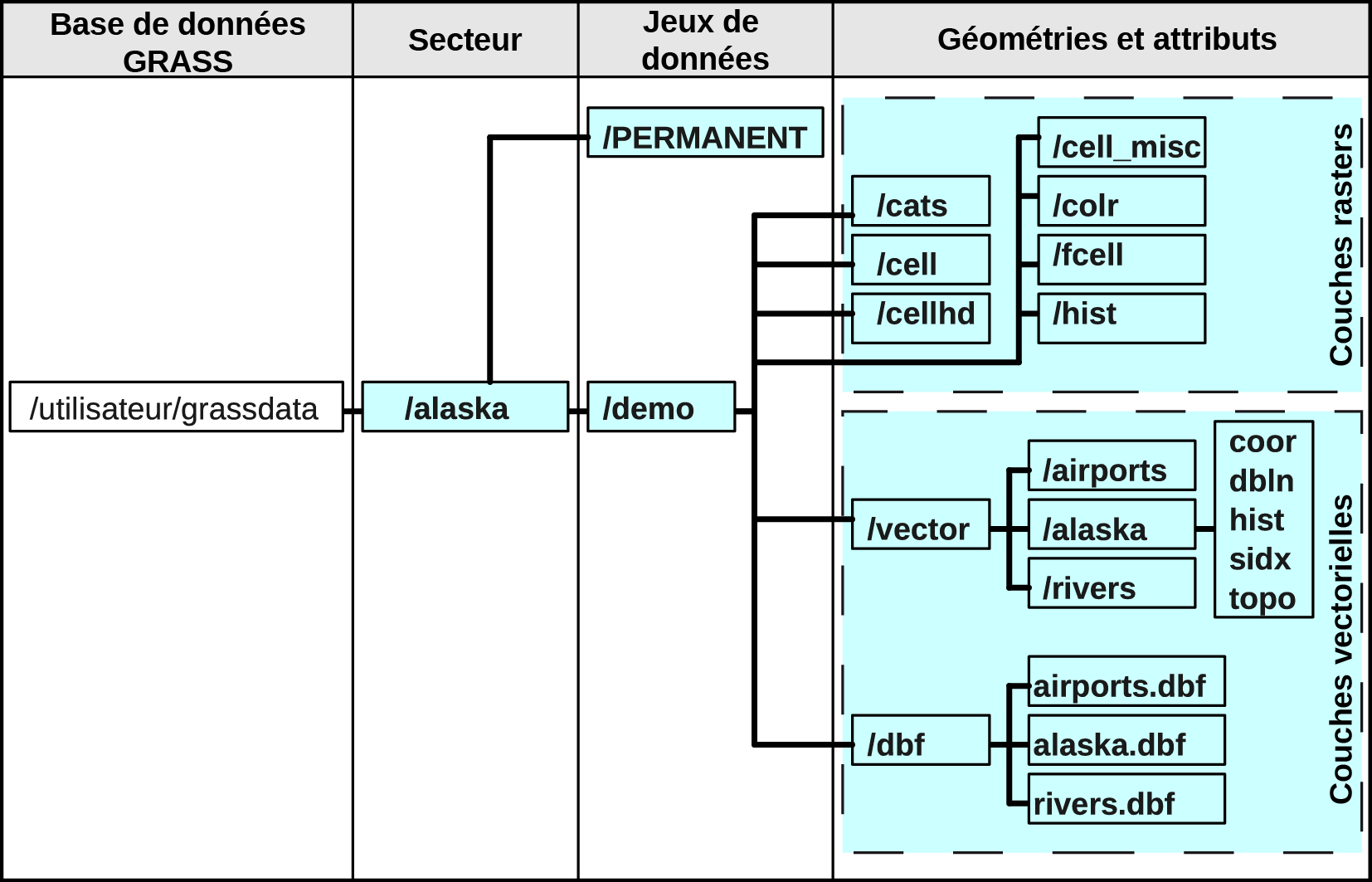
Données GRASS du SECTEUR Alaska

Créer un nouveau SECTEUR GRASS¶

As an example, here is how the sample GRASS LOCATION alaska, which is projected in Albers Equal Area projection with unit feet was created for the QGIS sample dataset. This sample GRASS LOCATION alaska will be used for all examples and exercises in the following GRASS-related sections. It is useful to download and install the dataset on your computer (see Échantillon de données).

1. Start QGIS and make sure the GRASS plugin is loaded.
2. Visualize the alaska.shp shapefile (see section Loading a Shapefile) from the QGIS Alaska dataset (see Échantillon de données).
3. In the GRASS toolbar, click on the ^{New mapset} icon to bring up the MAPSET wizard.

4. Sélectionnez un répertoire existant de base de données GRASS (GISDBASE) grassdata ou créez en un pour le nouveau SECTEUR avec le gestionnaire de fichiers de votre ordinateur. Cliquez sur le bouton [Suivant].

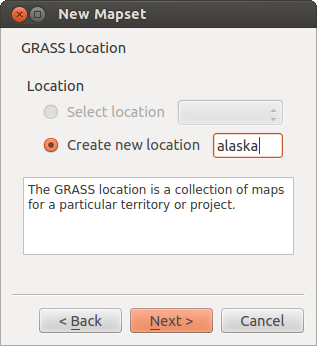
5. We can use this wizard to create a new MAPSET within an existing LOCATION (see section Ajouter un nouveau Jeu de données) or to create a new LOCATION altogether. Select Create new location (see figure_grass_location_2).

6. Entrez un nom pour le SECTEUR – nous avons utilisé ‘alaska’ – et cliquez sur le bouton [Suivant].

7. Define the projection by clicking on the radio button Projection to enable the projection list.
8. We are using Albers Equal Area Alaska (feet) projection. Since we happen to know that it is represented by the EPSG ID 2964, we enter it in the search box. (Note: If you want to repeat this process for another LOCATION and projection and haven’t memorized the EPSG ID, click on the ^{CRS Status} icon in the lower right-hand corner of the status bar (see section Utiliser les projections)).

9. Saisissez 2964 dans le Filtre pour sélectionner la projection.

10. Cliquez sur [Suivant].

11. To define the default region, we have to enter the LOCATION bounds in the north, south, east, and west directions. Here, we simply click on the button [Set current |qg| extent], to apply the extent of the loaded layer alaska.shp as the GRASS default region extent.

12. Cliquez sur [Suivant].

13. Nous avons aussi besoin de définir un Jeu de données dans notre nouveau SECTEUR (étape indispensable lors de la création d’un nouveau SECTEUR). Vous pouvez l’appeler comme vous le souhaitez - nous utiliserons ‘demo’. GRASS crée automatiquement un Jeu de données spécial appelé PERMANENT, conçu pour stocker les données essentielles du projet, son emprise spatiale par défaut et la définition du système de coordonnées (voir Neteler & Mitasova 2008 Bibliographie).

14. Vérifiez le résumé pour vous assurez que tout est correct et cliquez sur [Terminer].

15. Le nouveau SECTEUR ‘alaska’ et les deux Jeux de données ‘démo’ et ‘PERMANENT’ sont créés. Le jeu de données ouvert à ce moment est ‘démo’, tel que vous l’avez défini.

16. Notez que certains outils de la barre d’outils GRASS qui n’étaient pas accessibles le sont maintenant.

Figure GRASS location 2:

Creating a new GRASS LOCATION or a new MAPSET in QGIS

If that seemed like a lot of steps, it’s really not all that bad and a very quick way to create a LOCATION. The LOCATION ‘alaska’ is now ready for data import (see section Importer des données dans un SECTEUR GRASS). You can also use the already-existing vector and raster data in the sample GRASS LOCATION ‘alaska’, included in the QGIS ‘Alaska’ dataset Échantillon de données, and move on to section Le modèle vecteur de GRASS.

Importer des données dans un SECTEUR GRASS¶

This section gives an example of how to import raster and vector data into the ‘alaska’ GRASS LOCATION provided by the QGIS ‘Alaska’ dataset. Therefore, we use the landcover raster map landcover.img and the vector GML file lakes.gml from the QGIS ‘Alaska’ dataset (see Échantillon de données).

1. Start QGIS and make sure the GRASS plugin is loaded.
2. In the GRASS toolbar, click the ^{Open MAPSET} icon to bring up the MAPSET wizard.
3. Select as GRASS database the folder grassdata in the QGIS Alaska dataset, as LOCATION ‘alaska’, as MAPSET ‘demo’ and click [OK].
4. Now click the ^{Open GRASS tools} icon. The GRASS Toolbox (see section La Boîte à outils GRASS) dialog appears.

5. Pour importer la couche raster landcover.img, cliquez sur le module r.in.gdal dans l’onglet Arborescence des modules. Ce module GRASS vous permet d’importer les fichiers raster gérés par la librairie GDAL dans un SECTEUR GRASS. La fenêtre r.in.gdal apparaît.

6. Browse to the folder raster in the QGIS ‘Alaska’ dataset and select the file landcover.img.

7. Définissez landcover_grass comme nom de sortie pour le raster et cliquez sur [Lancer]. Dans l’onglet Rendu, vous voyez la commande GRASS en cours r.in.gdal -o input=/path/to/landcover.img output=landcover_grass.

8. When it says Succesfully finished, click [View output]. The landcover_grass raster layer is now imported into GRASS and will be visualized in the QGIS canvas.

9. Pour importer le fichier GML lakes.gml, cliquez sur le module v.in.ogr dans l’onglet Arborescence des modules. Ce module vous permet d’importer des données vectorielles gérées par OGR dans un SECTEUR GRASS. La fenêtre v.in.ogr apparaît.

10. Browse to the folder gml in the QGIS ‘Alaska’ dataset and select the file lakes.gml as OGR file.

11. Définissez lakes_grass comme nom de sortie et cliquez sur [Lancer]. Vous n’avez pas besoin des autres options dans cet exemple. Dans l’onglet Rendu, vous voyez la commande GRASS en cours v.in.ogr -o dsn=/path/to/lakes.gml output=lakes\_grass.

12. When it says Succesfully finished, click [View output]. The lakes_grass vector layer is now imported into GRASS and will be visualized in the QGIS canvas.

Le modèle vecteur de GRASS¶

It is important to understand the GRASS vector data model prior to digitizing.

In general, GRASS uses a topological vector model.

This means that areas are not represented as closed polygons, but by one or more boundaries. A boundary between two adjacent areas is digitized only once, and it is shared by both areas. Boundaries must be connected and closed without gaps. An area is identified (and labeled) by the centroid of the area.

Outre les limites et centroïdes, une couche vectorielle peut également contenir des points et des lignes. Tous ces éléments de géométrie peuvent être mélangés dans une couche vectorielle et seront représentés dans différentes ‘sous-couches’ dans une carte vectorielle GRASS. Ainsi, une couche GRASS n’est pas un vecteur ou un raster, mais un niveau à l’intérieur d’une couche vectorielle. Il est important de bien distinguer ceci (même s’il est possible de mélanger des éléments de géométries différentes, c’est inhabituel et même dans GRASS, on l’utilise dans des cas particuliers tel que l’analyse de réseau. Normalement, vous devriez stocker des éléments de géométries différentes dans des couches différentes).

Il est possible de stocker plusieurs ‘sous-couches’ dans une couche vectorielle. Par exemple, des champs, de la forêt et des lacs peuvent être stockés dans une couche vectorielle. Des forêts et des lacs adjacents partagent les mêmes limites, mais ils auront des tables attributaires différentes. Il est aussi possible de faire correspondre une table attributaire aux limites. Par exemple, la limite entre un lac et une forêt peut être une route qui peut avoir une table attributaire différente.

La ‘sous-couche’ est définie dans GRASS par un chiffre. Ce chiffre définit s’il y a plusieurs sous-couches à l’intérieur d’une couche vectorielle (par exemple, il définit s’il s’agit de lac ou de forêt). Pour l’instant, il s’agit d’un nombre, mais dans des versions futures GRASS pourra utiliser des noms pour les sous-couches dans l’interface utilisateur.

Attributes can be stored inside the GRASS LOCATION as dBase or SQLite3 or in external database tables, for example, PostgreSQL, MySQL, Oracle, etc.

Les données attributaires sont liées à la géométrie par le biais d’un champ ‘category’.

‘Category’ (clé, ID) est un entier attaché à la géométrie, et il est utilisé comme lien vers une colonne de clé dans la table de base de données.

Création d’une nouvelle couche vectorielle GRASS¶

To create a new GRASS vector layer with the GRASS plugin, click the ^{Create new GRASS vector} toolbar icon. Enter a name in the text box, and you can start digitizing point, line or polygon geometries following the procedure described in section Numérisation et édition de couche vectorielle GRASS.

In GRASS, it is possible to organize all sorts of geometry types (point, line and area) in one layer, because GRASS uses a topological vector model, so you don’t need to select the geometry type when creating a new GRASS vector. This is different from shapefile creation with QGIS, because shapefiles use the Simple Feature vector model (see section Créer de nouvelles couches vecteur).

Numérisation et édition de couche vectorielle GRASS¶

The digitizing tools for GRASS vector layers are accessed using the ^{Edit GRASS vector layer} icon on the toolbar. Make sure you have loaded a GRASS vector and it is the selected layer in the legend before clicking on the edit tool. Figure figure_grass_digitizing_2 shows the GRASS edit dialog that is displayed when you click on the edit tool. The tools and settings are discussed in the following sections.

Barre d’outils

In figure_grass_digitizing_1, you see the GRASS digitizing toolbar icons provided by the GRASS plugin. Table table_grass_digitizing_1 explains the available functionalities.

Figure GRASS digitizing 1:

GRASS Digitizing Toolbar

Icône	Outil	Fonction
	Nouveau Point	Numérise un nouveau point
	Nouvelle Ligne	Numérise une nouvelle ligne
	Nouveau Contour	Digitize new boundary (finish by selecting new tool)
	Nouveau Centroïde	Numérise un nouveau centroïde (permet d’étiqueter un polygone existant)
	Move vertex	Move one vertex of existing line or boundary and identify new position
	Add vertex	Add a new vertex to existing line
	Delete vertex	Delete vertex from existing line (confirm selected vertex by another click)
	Move element	Move selected boundary, line, point or centroid and click on new position
	Split line	Split an existing line into two parts
	Delete element	Delete existing boundary, line, point or centroid (confirm selected element by another click)
	Edit attributes	Edit attributes of selected element (note that one element can represent more features, see above)
	Close	Close session and save current status (rebuilds topology afterwards)

Tableau Numérisation avec GRASS 1 : outils d’édition GRASS

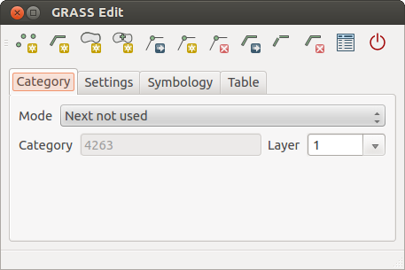
Category Tab

The Category tab allows you to define the way in which the category values will be assigned to a new geometry element.

Figure GRASS digitizing 2:

GRASS Digitizing Category Tab

• Mode: The category value that will be applied to new geometry elements.
  • Next not used - Apply next not yet used category value to geometry element.
  • Manual entry - Manually define the category value for the geometry element in the ‘Category’ entry field.
  • No category - Do not apply a category value to the geometry element. This is used, for instance, for area boundaries, because the category values are connected via the centroid.
• Category - The number (ID) that is attached to each digitized geometry element. It is used to connect each geometry element with its attributes.
• Field (layer) - Each geometry element can be connected with several attribute tables using different GRASS geometry layers. The default layer number is 1.

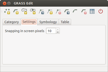
Settings Tab

The Settings tab allows you to set the snapping in screen pixels. The threshold defines at what distance new points or line ends are snapped to existing nodes. This helps to prevent gaps or dangles between boundaries. The default is set to 10 pixels.

Figure GRASS digitizing 3:

GRASS Digitizing Settings Tab

Symbology Tab

The Symbology tab allows you to view and set symbology and color settings for various geometry types and their topological status (e.g., closed / opened boundary).

Figure GRASS digitizing 4:

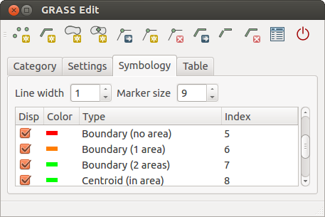
GRASS Digitizing Symbology Tab

Table Tab

The Table tab provides information about the database table for a given ‘layer’. Here, you can add new columns to an existing attribute table, or create a new database table for a new GRASS vector layer (see section Création d’une nouvelle couche vectorielle GRASS).

Figure GRASS digitizing 5:

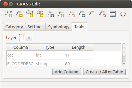
GRASS Digitizing Table Tab

L’outil région GRASS¶

La définition d’une région (définir une emprise spatiale de travail) dans GRASS est très importante pour travailler avec des couches rasters. Le travail d’analyse vecteur n’est, par défaut, pas limitée à une région définie. Mais, tous les rasters nouvellement créés auront l’emprise spatiale et la résolution de la région GRASS en cours d’utilisation, indépendamment de leur emprise et résolution d’origine. La région courante GRASS est stockée dans le fichier $LOCATION/$MAPSET/WIND, et celui-ci définit les limites Nord, Sud, Est et Ouest, le nombre de lignes et de colonnes ainsi que la résolution spatiale horizontale et verticale.

It is possible to switch on and off the visualization of the GRASS region in the QGIS canvas using the ^{Display current GRASS region} button.

With the ^{Edit current GRASS region} icon, you can open a dialog to change the current region and the symbology of the GRASS region rectangle in the QGIS canvas. Type in the new region bounds and resolution, and click [OK]. The dialog also allows you to select a new region interactively with your mouse on the QGIS canvas. Therefore, click with the left mouse button in the QGIS canvas, open a rectangle, close it using the left mouse button again and click [OK].

Le module GRASS g.region propose un grand nombre de paramètres pour définir de façon appropriée les limites et la résolution d’une région pour faire de l’analyse raster. Vous pouvez vous servir de ces paramètres dans la boîte à outils GRASS décrite dans la section La Boîte à outils GRASS.

La Boîte à outils GRASS¶

The ^{Open GRASS Tools} box provides GRASS module functionalities to work with data inside a selected GRASS LOCATION and MAPSET. To use the GRASS Toolbox you need to open a LOCATION and MAPSET that you have write permission for (usually granted, if you created the MAPSET). This is necessary, because new raster or vector layers created during analysis need to be written to the currently selected LOCATION and MAPSET.

Figure GRASS Toolbox 1:

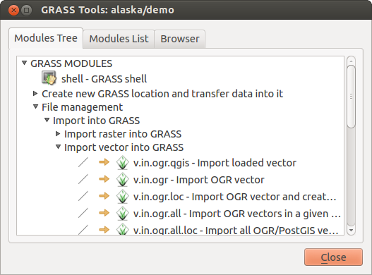
La Boîte à outils GRASS et la l’Arborescence des modules

Travailler avec les modules GRASS¶

La console de la Boîte à outils GRASS vous donne accès à pratiquement tous les modules GRASS (plus de 300) en ligne de commande. Afin d’offrir un environnement de travail plus agréable, environ 200 d’entre eux sont disponibles via l’interface graphique de la Boîte à outils GRASS.

A complete list of GRASS modules available in the graphical Toolbox in QGIS version 2.8 is available in the GRASS wiki at http://grass.osgeo.org/wiki/GRASS-QGIS_relevant_module_list.

Il est aussi possible de personnaliser le contenu de la boîte à outils GRASS. Ceci est décrit dans la section Paramètrer la boîte à outils GRASS.

Comme indiqué sur la figure figure_grass_toolbox_1, vous pouvez chercher le module GRASS approprié en utilisant l’onglet Arborescence des modules ou en utilisant l’onglet Liste des Modules pour faire une recherche.

Lorsque vous cliquez sur un module, un nouvel onglet apparaît proposant trois sous-onglets : Options, Rendu et Manuel.

Options

The Options tab provides a simplified module dialog where you can usually select a raster or vector layer visualized in the QGIS canvas and enter further module-specific parameters to run the module.

Figure GRASS module 1:

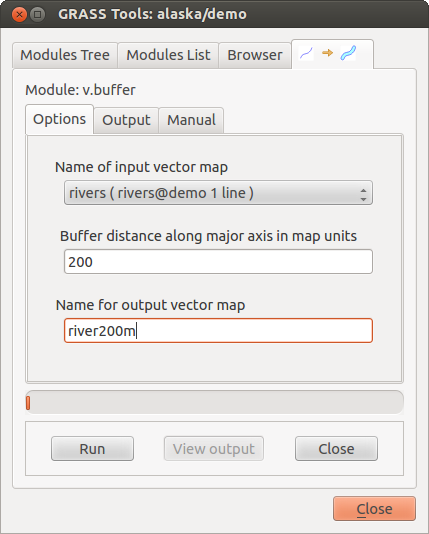
Boîte à outils GRASS, onglet Options d’un module

The provided module parameters are often not complete to keep the dialog clear. If you want to use further module parameters and flags, you need to start the GRASS shell and run the module in the command line.

A new feature since QGIS 1.8 is the support for a Show Advanced Options button below the simplified module dialog in the Options tab. At the moment, it is only added to the module v.in.ascii as an example of use, but it will probably be part of more or all modules in the GRASS Toolbox in future versions of QGIS. This allows you to use the complete GRASS module options without the need to switch to the GRASS shell.

Rendu

Figure GRASS module 2:

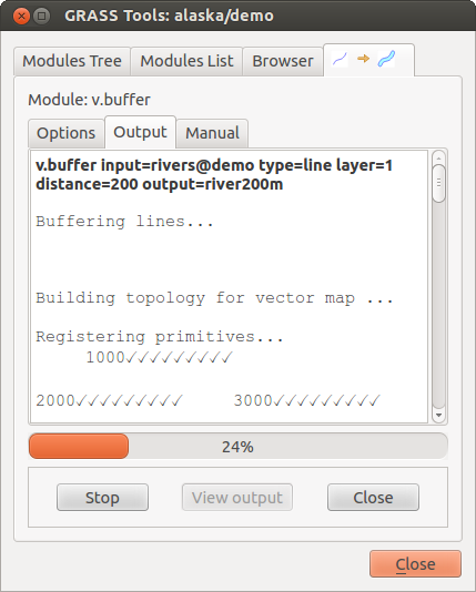
Boîte à outils GRASS, onglet Sortie d’un module

L’onglet Rendu fournit des informations sur l’état de sortie du module. Quand vous cliquez sur le bouton [Lancer], le module passe sur l’onglet Rendu et vous voyez les informations sur le processus en cours. Si tout se passe bien, vous verrez finalement le message Terminé avec succès.

Manuel

Figure GRASS module 3:

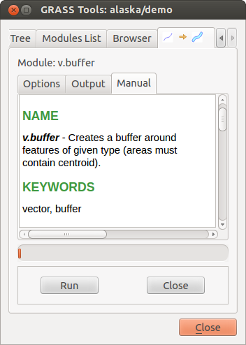
Boîte à outils GRASS, onglet Manuel d’un module

L’onglet Manuel montre la page HTML d’aide du module GRASS. Vous pouvez vous en servir pour voir les autres paramètres du module et pour avoir une connaissance plus approfondie de l’objet du module. À la fin de chaque page d’aide d’un module, vous avez des liens vers Main Help index (index principal), Thematic.index (index par thème) et Full.index (index complet). Ces liens vous donnent les mêmes informations que si vous utilisiez directement g.manual.

Astuce

Afficher les résultats immédiatement

Si vous voulez voir immédiatement dans votre fenêtre carte le résultat des calculs du module, vous pouvez utiliser le bouton ‘Vue’ au bas de l’onglet du module.

Exemples de modules GRASS¶

Les exemples suivants décrivent les possibilités de certains modules GRASS.

Création de courbes de niveau¶

Le premier exemple permet de créer une couche vectorielle de courbes de niveau à partir d’un modèle numérique de terrain (MNT). Ici, nous considérerons que le SECTEUR Alaska a été installé comme décrit dans la section Importer des données dans un SECTEUR GRASS.

• First, open the location by clicking the ^{Open mapset} button and choosing the Alaska location.
• Now load the gtopo30 elevation raster by clicking ^{Add GRASS raster layer} and selecting the gtopo30 raster from the demo location.
• Now open the Toolbox with the ^{Open GRASS tools} button.

• Dans la liste des outils double-cliquez sur Raster -> Gestion de surface -> Générer des lignes vectorielles de contours.

• Now a single click on the tool r.contour will open the tool dialog as explained above (see Travailler avec les modules GRASS). The gtopo30 raster should appear as the Name of input raster.
• Type into the Increment between Contour levels the value 100. (This will create contour lines at intervals of 100 meters.)

• Saisisez dans le champ Nom de la couche vectorielle en sortie, le nom ctour_100.

• Cliquer sur [Lancer] pour lancer le traitement. Attendez quelques instants que le message Terminé avec succès apparaisse à l’écran. Cliquez enfin sur [Vue] puis [Fermer].

Comme il s’agit d’une grande région, cela prendra un certain temps à s’afficher. Une fois l’affichage terminé, vous pouvez ouvrir la fenêtre de propriétés de la couche pour changer la couleur des courbes de niveau afin qu’elles apparaissent clairement au dessus de la couche raster d’élévation comme décrit dans Fenêtre Propriétés d’une couche vecteur.

Zoomez sur une petite région montagneuse du centre de l’Alaska. Avec un zoom important, vous constaterez que les courbes de niveau sont constituées de lignes brisées avec des angles vifs. GRASS offre la possibilité de généraliser les cartes vecteurs à l’aide de l’outil v.generalize, tout en conservant leur forme générale. L’outil utilise différents algorithmes ayant différents objectifs. Certains de ces algorithmes (par exemple : Douglas Peucker et Réduction de Vertex) simplifient les lignes en supprimant des sommets. La couche simplifiée se chargera plus rapidement. Cette commande est utile lorsque vous avez une couche vectorielle très détaillée et que vous créez une carte à petite échelle où les détails ne sont donc pas nécessaires.

Astuce

L’outil de simplification

Note that the QGIS fTools plugin has a Simplify geometries ‣ tool that works just like the GRASS v.generalize Douglas-Peuker algorithm.

Cependant, le but de cet exemple est différent. Les courbes de niveau créées avec r.contour ont des angles vifs qui doivent être lissés. Parmi les algorithmes de v.generalize, il y a l’algorithme de Chaiken qui fait justement ça (comme Hermite splines). Gardez à l’esprit que ces algorithmes peuvent ajouter des sommets supplémentaires au vecteur, l’amenant à se charger encore plus lentement.

• Ouvrez la Boîte à outils GRASS et double cliquez sur Vecteur -> Développer la carte -> Généralisation. Cliquez alors sur le module v.generalize pour ouvrir sa fenêtre d’options.

• rifier que la couche vectorielle ‘ctour_100’ apparait dans le champ Nom de la couche vectorielle en entrée.

• Dans la liste des algorithmes choisissez Chaiken. Laisser les autres options par défaut et descendez à la dernière ligne pour donner le nom de la couche d’information à créer : Nom de la couche vectorielle en sortie ‘ctour_100_smooth’, et cliquez sur [Lancer].

• Cela peut prendre plusieurs minutes. Lorsque le texte Terminé avec succès apparait, cliquez sur le bouton [Vue] puis sur [Fermer].

• Vous pouvez changer la couleur de cette couche vectorielle pour qu’elle apparaisse clairement sur le raster et qu’elle contraste aussi avec la couche de départ.Vous remarquerez que les nouvelles courbes de niveau ont des angles plus arrondis que l’original tout en restant fidèle à la forme globale d’origine.

Figure GRASS module 4:

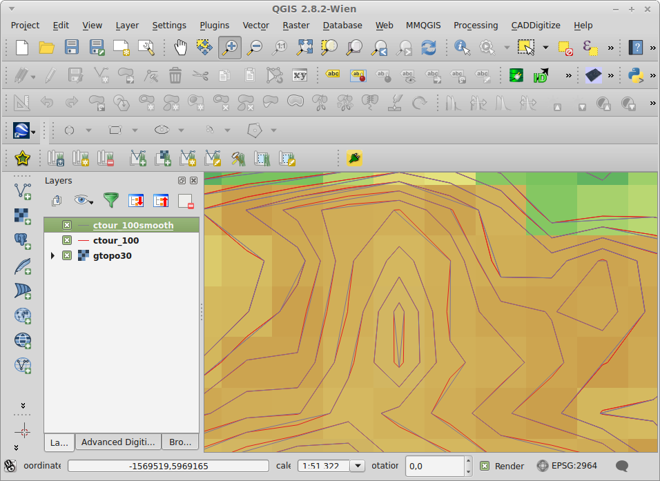
Module GRASS v.generalize utilisé pour simplifier une couche vectorielle

Astuce

Autres utilisations de r.contour

La procédure décrite ci-dessus peut être utilisée dans d’autres cas similaires. Si vous disposez d’une couche d’informations raster représentant des précipitations, par exemple, vous pouvez utiliser la même méthode pour créer des isohyètes (lignes reliant des points d’égales quantités de précipitations).

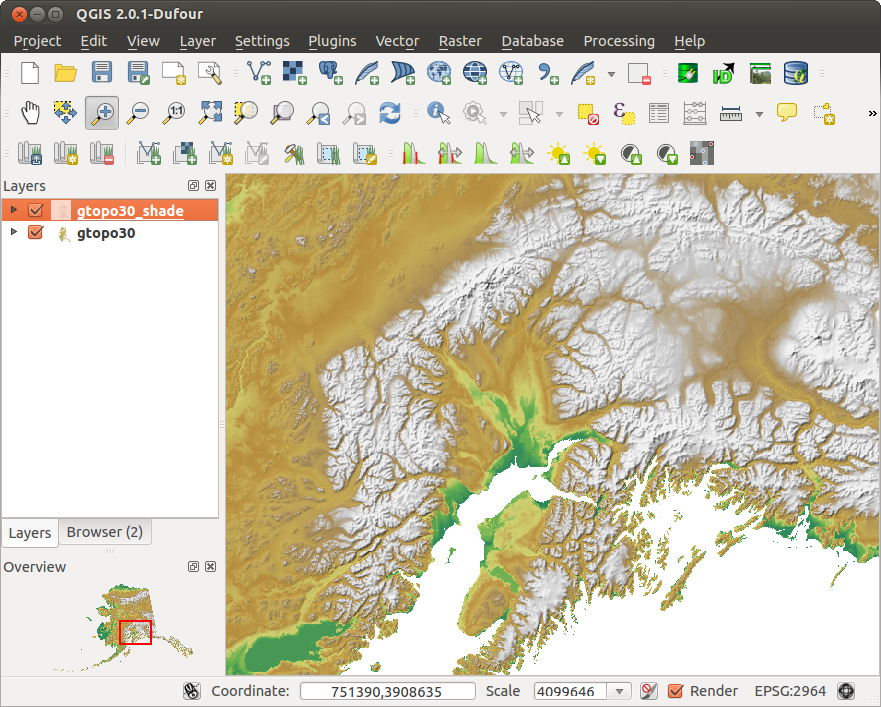
Créer un ombrage avec effet 3D¶

Différentes méthodes sont utilisées pour afficher les modèles numérique de terrain et donner un effet 3D au carte. L’utilisation de courbes de niveau comme décrit ci-dessus est un des moyens souvent utilisés pour produire des cartes topographiques. Un autre moyen de rendre cet effet 3D est d’utiliser l’ombrage. L’ombrage est créé à partir du modèle numérique de terrain (MNT) en calculant d’abord les pentes et les expositions puis en simulant la position du soleil dans le ciel ce qui donne à chaque cellule une valeur de réflectance. Les pentes éclairées par le soleil sont plus claires et les pentes à l’abri du soleil sont plus sombres.

• Commencez par ouvrir la couche raster gtopo30. Ouvrez la Boîte à outils GRASS et dans la catégorie Raster double cliquez sur Analyse spatiale ‣ Analyse de terrain.

• Cliquez ensuite sur r.shaded.relief pour lancer le module.

• Change the azimuth angle 270 to 315.

• Saisissez gtopo30_shade comme nom pour la nouvelle couche d’ombrage et cliquez sur le bouton [Lancer].

• Quand le calcul est terminé, ajoutez le raster d’ombrage à la fenêtre carte. Normalement, il devrait s’afficher en niveau de gris.

• Pour voir les deux couches d’informations ombrage et gtopo30 en même temps, placez la couche ombrage sous la couche gtopo30 dans le gestionnaire de couches et ouvrez la fenêtre Propriétés de la couche gtopo30, allez sur l’onglet Transparence et fixez la transparence à environ 25%.

Vous devriez maintenant avoir la couche gtopo30 en couleur et en transparence, affiché au dessus de la couche d’ombrage en niveau de gris. Pour bien visualiser l’effet d’ombrage, décochez puis recochez la couche gtopo30_shade dans la légende.

Utiliser la console GRASS

The GRASS plugin in QGIS is designed for users who are new to GRASS and not familiar with all the modules and options. As such, some modules in the Toolbox do not show all the options available, and some modules do not appear at all. The GRASS shell (or console) gives the user access to those additional GRASS modules that do not appear in the Toolbox tree, and also to some additional options to the modules that are in the Toolbox with the simplest default parameters. This example demonstrates the use of an additional option in the r.shaded.relief module that was shown above.

Figure GRASS module 5:

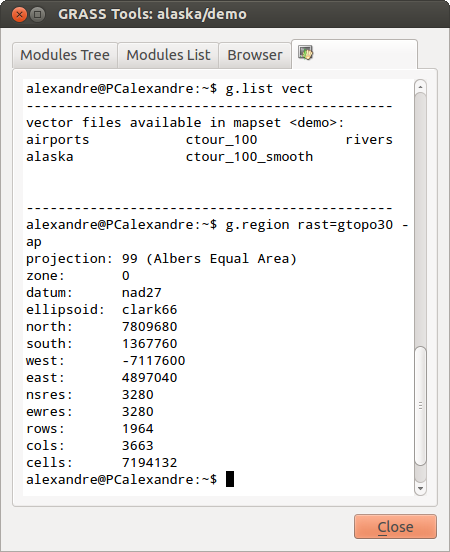
La console GRASS utilisation du module r.shaded.relief

Le module r.shaded.relief possède un paramètre zmult qui multiplie la valeur de l’altitude (exprimé dans la même unité que les coordonnées X - Y) ce qui a pour effet d’accentuer le relief.

• Ouvrez le raster gtopo30 comme ci-dessus, lancez la Boîte à outils GRASS et ouvrez la console GRASS. Dans la console, entrez la ligne suivante r.shaded.relief map=gtopo30 shade=gtopo30_shade2 azimuth=315 zmult=3 et pressez [Entrée].

• After the process finishes, shift to the Browse tab and double-click on the new gtopo30_shade2 raster to display it in QGIS.

• Comme expliqué ci-dessus, placez le raster d’ombrage sous le raster gtopo30 puis vérifiez la transparence du raster gtopo30. Vous devriez constater que le relief apparaît plus marqué qu’avec le premier raster d’ombrage.

Figure GRASS module 6:

Affichage du relief ombré créé avec le module GRASS r.shaded.relief

Statistiques raster avec des couches vectorielles¶

L’exemple suivant comment un module GRASS peut aggréger des données raster et ajouter des colonnes de statistiques pour chaque polygone d’une couche vectorielle.

• Encore une fois, nous allons utiliser le jeu de données Alaska. Référez vous à Importer des données dans un SECTEUR GRASS pour importer les shapefiles contenus dans le répetoire shapefiles dans GRASS.

• Un étape intermédiaire est nécessaire : des centroïdes doivent importés afin d’avoir une couche GRASS vecteur complète (qui inclue les contours et les centroïdes).

• Dans la Boîte à outils choisissez Vecteur -> Gestion des entités et ouvrez le module v.centroids.

• Entrez ‘forest_areas’ comme nom de couche en sortie et lancez le module.

• Now load the forest_areas vector and display the types of forests - deciduous, evergreen, mixed - in different colors: In the layer Properties window, Symbology tab, choose from Legend type ‘Unique value’ and set the Classification field to ‘VEGDESC’. (Refer to the explanation of the symbology tab in Onglet Style of the vector section.)

• Réouvrez la Boîte à outils GRASS et ouvrez Vecteur -> Mise à jour vectorielle via d’autres cartes.

• Cliquez sur le module v.rast.stats. Saisissez gtopo30 et forest_areas.

• Un seul paramètre additionnel est requis : Entrez elev pour le column prefix, et cliquez sur le bouton [Lancer]. C’est un opération lourde qui peut durer longtemps (jusqu’à deux heures).

• Pour finir, ouvrez la table attributaire de forest_areas, et vérifiez que plusieurs nouvelles colonnes ont étés ajoutées dont elev_min, elev_max, elev_mean, etc., pour chaque polygone de forêt.

Working with the GRASS LOCATION browser¶

Another useful feature inside the GRASS Toolbox is the GRASS LOCATION browser. In figure_grass_module_7, you can see the current working LOCATION with its MAPSETs.

In the left browser windows, you can browse through all MAPSETs inside the current LOCATION. The right browser window shows some meta-information for selected raster or vector layers (e.g., resolution, bounding box, data source, connected attribute table for vector data, and a command history).

Figure GRASS module 7:

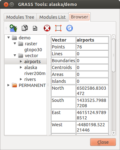
GRASS LOCATION browser

The toolbar inside the Browser tab offers the following tools to manage the selected LOCATION:

• Add selected map to canvas
• Copy selected map
• Rename selected map
• Delete selected map
• Set current region to selected map
• Refresh browser window

The Rename selected map and Delete selected map only work with maps inside your currently selected MAPSET. All other tools also work with raster and vector layers in another MAPSET.

<?xml version="1.0" encoding="UTF-8"?>
<!DOCTYPE qgisgrassmodule SYSTEM "http://mrcc.com/qgisgrassmodule.dtd">

<qgisgrassmodule label="Vector buffer" module="v.buffer">
        <option key="input" typeoption="type" layeroption="layer" />
        <option key="buffer"/>
        <option key="output" />
</qgisgrassmodule>