.
The toolbox
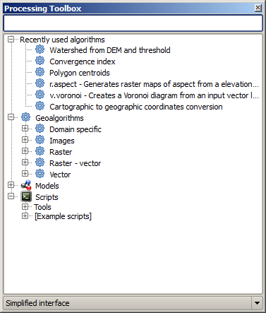
The Toolbox is the main element of the processing GUI, and the one that you are more likely to use in your daily work. It shows the list of all available algorithms grouped in different blocks, and it is the access point to run them, whether as a single process or as a batch process involving several executions of the same algorithm on different sets of inputs.
Figure Processing 5:
Processing Toolbox 
The toolbox contains all the available algorithms, divided into predefined groups. All these groups are found under a single tree entry named Geoalgorithms.
Additionally, two more entries are found, namely Models and Scripts. These include user-created algorithms, and they allow you to define your own workflows and processing tasks. We will devote a full section to them a bit later.
In the upper part of the toolbox, you will find a text box. To reduce the number of algorithms shown in the toolbox and make it easier to find the one you need, you can enter any word or phrase on the text box. Notice that, as you type, the number of algorithms in the toolbox is reduced to just those that contain the text you have entered in their names.
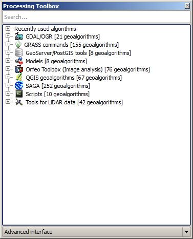
In the lower part, you will find a box that allows you to switch between the simplified algorithm list (the one explained above) and the advanced list. If you change to the advanced mode, the toolbox will look like this:
Figure Processing 6:
Processing Toolbox (advanced mode)
In the advanced view, each group represents a so-called ‘algorithm provider’, which is a set of algorithms coming from the same source, for instance, from a third-party application with geoprocessing capabilities. Some of these groups represent algorithms from third-party applications like SAGA, GRASS or R, while others contain algorithms directly coded as part of the processing plugin, not relying on any additional software.
This view is recommended to those users who have a certain knowledge of the applications that are backing the algorithms, since they will be shown with their original names and groups.
Also, some additional algorithms are available only in the advanced view, such as LiDAR tools and scripts based on the R statistical computing software, among others. Independent QGIS plugins that add new algorithms to the toolbox will only be shown in the advanced view.
In particular, the simplified view contains algorithms from the following providers:
- GRASS
- SAGA
- OTB
- Native QGIS algorithms
In the case of running QGIS under Windows, these algorithms are fully-functional in a fresh installation of QGIS, and they can be run without requiring any additional installation. Also, running them requires no prior knowledge of the external applications they use, making them more accesible for first-time users.
If you want to use an algorithm not provided by any of the above providers, switch to the advanced mode by selecting the corresponding option at the bottom of the toolbox.
To execute an algorithm, just double-click on its name in the toolbox.
The algorithm dialog
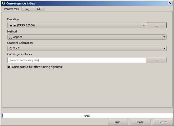
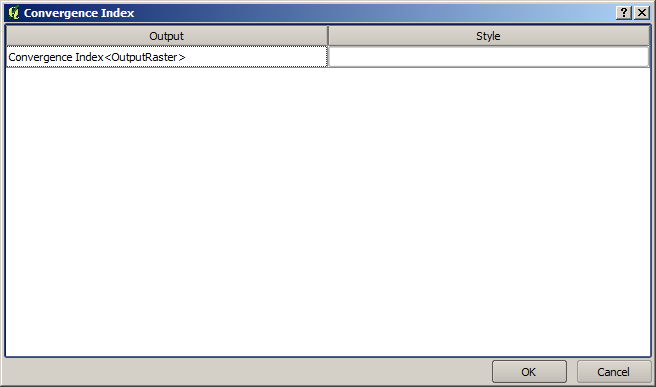
Once you double-click on the name of the algorithm that you want to execute, a dialog similar to that in the figure below is shown (in this case, the dialog corresponds to the SAGA ‘Convergence index’ algorithm).
Figure Processing 7:
Parameters Dialog
This dialog is used to set the input values that the algorithm needs to be executed. It shows a table where input values and configuration parameters are to be set. It of course has a different content, depending on the requirements of the algorithm to be executed, and is created automatically based on those requirements. On the left side, the name of the parameter is shown. On the right side, the value of the parameter can be set.
Although the number and type of parameters depend on the characteristics of the algorithm, the structure is similar for all of them. The parameters found in the table can be of one of the following types.
A raster layer, to select from a list of all such layers available (currently opened) in QGIS. The selector contains as well a button on its right-hand side, to let you select filenames that represent layers currently not loaded in QGIS.
A vector layer, to select from a list of all vector layers available in QGIS. Layers not loaded in QGIS can be selected as well, as in the case of raster layers, but only if the algorithm does not require a table field selected from the attributes table of the layer. In that case, only opened layers can be selected, since they need to be open so as to retrieve the list of field names available.
You will see a button by each vector layer selector, as shown in the figure below.
Figure Processing 8:
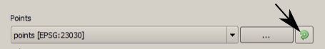
Vector iterator button
If the algorithm contains several of them, you will be able to toggle just one of them. If the button corresponding to a vector input is toggled, the algorithm will be executed iteratively on each one of its features, instead of just once for the whole layer, producing as many outputs as times the algorithm is executed. This allows for automating the process when all features in a layer have to be processed separately.
- A table, to select from a list of all available in QGIS. Non-spatial tables are loaded into QGIS like vector layers, and in fact they are treated as such by the program. Currently, the list of available tables that you will see when executing an algorithm that needs one of them is restricted to tables coming from files in dBase (.dbf) or Comma-Separated Values (.csv) formats.
- An option, to choose from a selection list of possible options.
- A numerical value, to be introduced in a text box. You will find a button by its side. Clicking on it, you will see a dialog that allows you to enter a mathematical expression, so you can use it as a handy calculator. Some useful variables related to data loaded into QGIS can be added to your expression, so you can select a value derived from any of these variables, such as the cell size of a layer or the northernmost coordinate of another one.
Figure Processing 9:
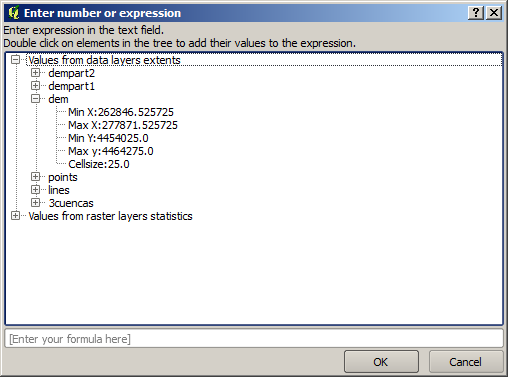
Number Selector
A range, with min and max values to be introduced in two text boxes.
A text string, to be introduced in a text box.
A field, to choose from the attributes table of a vector layer or a single table selected in another parameter.
A coordinate reference system. You can type the EPSG code directly in the text box, or select it from the CRS selection dialog that appears when you click on the button on the right-hand side.
An extent, to be entered by four numbers representing its xmin, xmax, ymin, ymax limits. Clicking on the button on the right-hand side of the value selector, a pop-up menu will appear, giving you two options: to select the value from a layer or the current canvas extent, or to define it by dragging directly onto the map canvas.
Figure Processing 10
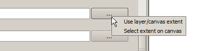
Extent selector
If you select the first option, you will see a window like the next one.
Figure Processing 11
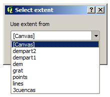
Extent List
If you select the second one, the parameters window will hide itself, so you can click and drag onto the canvas. Once you have defined the selected rectangle, the dialog will reappear, containing the values in the extent text box.
Figure Processing 12:
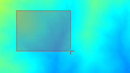
Extent Drag
A list of elements (whether raster layers, vector layers or tables), to select from the list of such layers available in QGIS. To make the selection, click on the small button on the left side of the corresponding row to see a dialog like the following one.
Figure Processing 13:
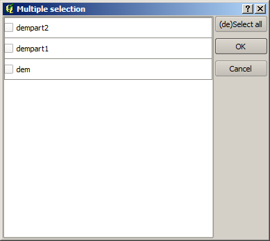
Multiple Selection
A small table to be edited by the user. These are used to define parameters like lookup tables or convolution kernels, among others.
Click on the button on the right side to see the table and edit its values.
Figure Processing 14:
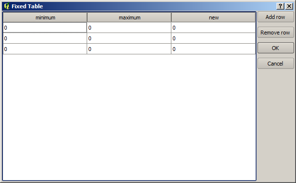
Fixed Table
Depending on the algorithm, the number of rows can be modified or not by using the buttons on the right side of the window.
You will find a [Help] tab in the the parameters dialog. If a help file is available, it will be shown, giving you more information about the algorithm and detailed descriptions of what each parameter does. Unfortunately, most algorithms lack good documentation, but if you feel like contributing to the project, this would be a good place to start.
A note on projections
Algorithms run from the processing framework — this is also true of most of the external applications whose algorithms are exposed through it. Do not perform any reprojection on input layers and assume that all of them are already in a common coordinate system and ready to be analized. Whenever you use more than one layer as input to an algorithm, whether vector or raster, it is up to you to make sure that they are all in the same coordinate system.
Note that, due to QGIS‘s on-the-fly reprojecting capabilities, although two layers might seem to overlap and match, that might not be true if their original coordinates are used without reprojecting them onto a common coordinate system. That reprojection should be done manually, and then the resulting files should be used as input to the algorithm. Also, note that the reprojection process can be performed with the algorithms that are available in the processing framework itself.
By default, the parameters dialog will show a description of the CRS of each layer along with its name, making it easy to select layers that share the same CRS to be used as input layers. If you do not want to see this additional information, you can disable this functionality in the processing configuration dialog, unchecking the Show CRS option.
If you try to execute an algorithm using as input two or more layers with unmatching CRSs, a warning dialog will be shown.
You still can execute the algorithm, but be aware that in most cases that will produce wrong results, such as empty layers due to input layers not overlapping.
Data objects generated by algorithms
Data objects generated by an algorithm can be of any of the following types:
- A raster layer
- A vector layer
- A table
- An HTML file (used for text and graphical outputs)
These are all saved to disk, and the parameters table will contain a text box corresponding to each one of these outputs, where you can type the output channel to use for saving it. An output channel contains the information needed to save the resulting object somewhere. In the most usual case, you will save it to a file, but the architecture allows for any other way of storing it. For instance, a vector layer can be stored in a database or even uploaded to a remote server using a WFS-T service. Although solutions like these are not yet implemented, the processing framework is prepared to handle them, and we expect to add new kinds of output channels in a near feature.
To select an output channel, just click on the button on the right side of the text box. That will open a save file dialog, where you can select the desired file path. Supported file extensions are shown in the file format selector of the dialog, depending on the kind of output and the algorithm.
The format of the output is defined by the filename extension. The supported formats depend on what is supported by the algorithm itself. To select a format, just select the corresponding file extension (or add it, if you are directly typing the file path instead). If the extension of the file path you entered does not match any of the supported formats, a default extension (usually .dbf` for tables, .tif for raster layers and .shp for vector layers) will be appended to the file path, and the file format corresponding to that extension will be used to save the layer or table.
If you do not enter any filename, the result will be saved as a temporary file in the corresponding default file format, and it will be deleted once you exit QGIS (take care with that, in case you save your project and it contains temporary layers).
You can set a default folder for output data objects. Go to the configuration dialog (you can open it from the Processing menu), and in the General group, you will find a parameter named Output folder. This output folder is used as the default path in case you type just a filename with no path (i.e., myfile.shp) when executing an algorithm.
When running an algorithm that uses a vector layer in iterative mode, the entered file path is used as the base path for all generated files, which are named using the base name and appending a number representing the index of the iteration. The file extension (and format) is used for all such generated files.
Apart from raster layers and tables, algorithms also generate graphics and text as HTML files. These results are shown at the end of the algorithm execution in a new dialog. This dialog will keep the results produced by any algorithm during the current session, and can be shown at any time by selecting Processing ‣ Results viewer from the QGIS main menu.
Some external applications might have files (with no particular extension restrictions) as output, but they do not belong to any of the categories above. Those output files will not be processed by QGIS (opened or included into the current QGIS project), since most of the time they correspond to file formats or elements not supported by QGIS. This is, for instance, the case with LAS files used for LiDAR data. The files get created, but you won’t see anything new in your QGIS working session.
For all the other types of output, you will find a checkbox that you can use to tell the algorithm whether to load the file once it is generated by the algorithm or not. By default, all files are opened.
Optional outputs are not supported. That is, all outputs are created. However, you can uncheck the corresponding checkbox if you are not interested in a given output, which essentially makes it behave like an optional output (in other words, the layer is created anyway, but if you leave the text box empty, it will be saved to a temporary file and deleted once you exit QGIS).
Configuring the processing framework
As has been mentioned, the configuration menu gives access to a new dialog where you can configure how algorithms work. Configuration parameters are structured in separate blocks that you can select on the left-hand side of the dialog.
Along with the aforementioned Output folder entry, the General block contains parameters for setting the default rendering style for output layers (that is, layers generated by using algorithms from any of the framework GUI components). Just create the style you want using QGIS, save it to a file, and then enter the path to that file in the settings so the algorithms can use it. Whenever a layer is loaded by SEXTANTE and added to the QGIS canvas, it will be rendered with that style.
Rendering styles can be configured individually for each algorithm and each one of its outputs. Just right-click on the name of the algorithm in the toolbox and select Edit rendering styles. You will see a dialog like the one shown next.
Figure Processing 15:
Rendering Styles
Select the style file (.qml) that you want for each output and press [OK].
Other configuration parameters in the General group are listed below:
- Use filename as layer name. The name of each resulting layer created by an algorithm is defined by the algorithm itself. In some cases, a fixed name might be used, meaning that the same output name will be used, no matter which input layer is used. In other cases, the name might depend on the name of the input layer or some of the parameters used to run the algorithm. If this checkbox is checked, the name will be taken from the output filename instead. Notice that, if the output is saved to a temporary file, the filename of this temporary file is usually a long and meaningless one intended to avoid collision with other already existing filenames.
- Use only selected features. If this option is selected, whenever a vector layer is used as input for an algorithm, only its selected features will be used. If the layer has no selected features, all features will be used.
- Pre-execution script file and Post-execution script file. These parameters refer to scripts written using the processing scripting functionality, and are explained in the section covering scripting and the console.
Apart from the General block in the settings dialog, you will also find a block for algorithm providers. Each entry in this block contains an Activate item that you can use to make algorithms appear or not in the toolbox. Also, some algorithm providers have their own configuration items, which we will explain later when covering particular algorithm providers.