GRASS GIS Integration¶

Starting the GRASS plugin¶

To use GRASS functionalities and/or visualize GRASS vector and raster layers in QGIS, you must select and load the GRASS plugin with the Plugin Manager. Therefore, go to the menu Plugins ‣ Manage Plugins, select GRASS and click [OK].

You can now start loading raster and vector layers from an existing GRASS LOCATION (see section sec_load_grassdata). Or, you can create a new GRASS LOCATION with QGIS (see section Creating a new GRASS LOCATION) and import some raster and vector data (see section Importing data into a GRASS LOCATION) for further analysis with the GRASS Toolbox (see section The GRASS Toolbox).

Loading GRASS raster and vector layers¶

With the GRASS plugin, you can load vector or raster layers using the appropriate button on the toolbar menu. As an example, we will use the QGIS Alaska dataset (see section Sample Data). It includes a small sample GRASS LOCATION with three vector layers and one raster elevation map.

1. Create a new folder called grassdata, download the QGIS ‘Alaska’ dataset qgis_sample_data.zip from http://download.osgeo.org/qgis/data/ and unzip the file into grassdata.
2. Start QGIS.
3. If not already done in a previous QGIS session, load the GRASS plugin clicking on Plugins ‣ Manage Plugins and activate GRASS. The GRASS toolbar appears in the QGIS main window.
4. In the GRASS toolbar, click the ^{Open mapset} icon to bring up the MAPSET wizard.
5. For Gisdbase, browse and select or enter the path to the newly created folder grassdata.
6. You should now be able to select the LOCATION alaska and the MAPSET demo.
7. Click [OK]. Notice that some previously disabled tools in the GRASS toolbar are now enabled.
8. Click on ^{Add GRASS raster layer}, choose the map name gtopo30 and click [OK]. The elevation layer will be visualized.
9. Click on ^{Add GRASS vector layer}, choose the map name alaska and click [OK]. The Alaska boundary vector layer will be overlayed on top of the gtopo30 map. You can now adapt the layer properties as described in chapter The Vector Properties Dialog (e.g., change opacity, fill and outline color).
10. Also load the other two vector layers, rivers and airports, and adapt their properties.

As you see, it is very simple to load GRASS raster and vector layers in QGIS. See the following sections for editing GRASS data and creating a new LOCATION. More sample GRASS LOCATIONs are available at the GRASS website at http://grass.osgeo.org/download/sample-data/.

GRASS LOCATION and MAPSET¶

GRASS data are stored in a directory referred to as GISDBASE. This directory, often called grassdata, must be created before you start working with the GRASS plugin in QGIS. Within this directory, the GRASS GIS data are organized by projects stored in subdirectories called LOCATIONs. Each LOCATION is defined by its coordinate system, map projection and geographical boundaries. Each LOCATION can have several MAPSETs (subdirectories of the LOCATION) that are used to subdivide the project into different topics or subregions, or as workspaces for individual team members (see Neteler & Mitasova 2008 in Literature and Web References). In order to analyze vector and raster layers with GRASS modules, you must import them into a GRASS LOCATION. (This is not strictly true – with the GRASS modules r.external and v.external you can create read-only links to external GDAL/OGR-supported datasets without importing them. But because this is not the usual way for beginners to work with GRASS, this functionality will not be described here.)

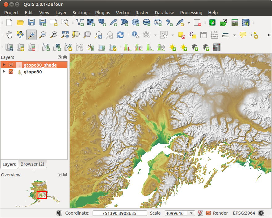
Figure GRASS location 1:

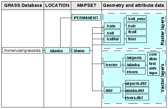
GRASS data in the alaska LOCATION

Creating a new GRASS LOCATION¶

As an example, here is how the sample GRASS LOCATION alaska, which is projected in Albers Equal Area projection with unit feet was created for the QGIS sample dataset. This sample GRASS LOCATION alaska will be used for all examples and exercises in the following GRASS-related sections. It is useful to download and install the dataset on your computer (see Sample Data).

1. Start QGIS and make sure the GRASS plugin is loaded.
2. Visualize the alaska.shp shapefile (see section Loading a Shapefile) from the QGIS Alaska dataset (see Sample Data).
3. In the GRASS toolbar, click on the ^{New mapset} icon to bring up the MAPSET wizard.
4. Select an existing GRASS database (GISDBASE) folder grassdata, or create one for the new LOCATION using a file manager on your computer. Then click [Next].
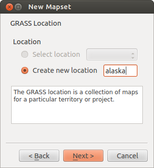
5. We can use this wizard to create a new MAPSET within an existing LOCATION (see section Adding a new MAPSET) or to create a new LOCATION altogether. Select Create new location (see figure_grass_location_2).
6. Enter a name for the LOCATION – we used ‘alaska’ – and click [Next].
7. Define the projection by clicking on the radio button Projection to enable the projection list.
8. We are using Albers Equal Area Alaska (feet) projection. Since we happen to know that it is represented by the EPSG ID 2964, we enter it in the search box. (Note: If you want to repeat this process for another LOCATION and projection and haven’t memorized the EPSG ID, click on the ^{CRS Status} icon in the lower right-hand corner of the status bar (see section Working with Projections)).
9. In Filter, insert 2964 to select the projection.
10. Click [Next].
11. To define the default region, we have to enter the LOCATION bounds in the north, south, east, and west directions. Here, we simply click on the button [Set current |qg| extent], to apply the extent of the loaded layer alaska.shp as the GRASS default region extent.
12. Click [Next].
13. We also need to define a MAPSET within our new LOCATION (this is necessary when creating a new LOCATION). You can name it whatever you like - we used ‘demo’. GRASS automatically creates a special MAPSET called PERMANENT, designed to store the core data for the project, its default spatial extent and coordinate system definitions (see Neteler & Mitasova 2008 in Literature and Web References).
14. Check out the summary to make sure it’s correct and click [Finish].
15. The new LOCATION, ‘alaska’, and two MAPSETs, ‘demo’ and ‘PERMANENT’, are created. The currently opened working set is ‘demo’, as you defined.
16. Notice that some of the tools in the GRASS toolbar that were disabled are now enabled.

Figure GRASS location 2:

Creating a new GRASS LOCATION or a new MAPSET in QGIS

If that seemed like a lot of steps, it’s really not all that bad and a very quick way to create a LOCATION. The LOCATION ‘alaska’ is now ready for data import (see section Importing data into a GRASS LOCATION). You can also use the already-existing vector and raster data in the sample GRASS LOCATION ‘alaska’, included in the QGIS ‘Alaska’ dataset Sample Data, and move on to section The GRASS vector data model.

Importing data into a GRASS LOCATION¶

This section gives an example of how to import raster and vector data into the ‘alaska’ GRASS LOCATION provided by the QGIS ‘Alaska’ dataset. Therefore, we use the landcover raster map landcover.img and the vector GML file lakes.gml from the QGIS ‘Alaska’ dataset (see Sample Data).

1. Start QGIS and make sure the GRASS plugin is loaded.
2. In the GRASS toolbar, click the ^{Open MAPSET} icon to bring up the MAPSET wizard.
3. Select as GRASS database the folder grassdata in the QGIS Alaska dataset, as LOCATION ‘alaska’, as MAPSET ‘demo’ and click [OK].
4. Now click the ^{Open GRASS tools} icon. The GRASS Toolbox (see section The GRASS Toolbox) dialog appears.
5. To import the raster map landcover.img, click the module r.in.gdal in the Modules Tree tab. This GRASS module allows you to import GDAL-supported raster files into a GRASS LOCATION. The module dialog for r.in.gdal appears.
6. Browse to the folder raster in the QGIS ‘Alaska’ dataset and select the file landcover.img.
7. As raster output name, define landcover_grass and click [Run]. In the Output tab, you see the currently running GRASS command r.in.gdal -o input=/path/to/landcover.img output=landcover_grass.
8. When it says Succesfully finished, click [View output]. The landcover_grass raster layer is now imported into GRASS and will be visualized in the QGIS canvas.
9. To import the vector GML file lakes.gml, click the module v.in.ogr in the Modules Tree tab. This GRASS module allows you to import OGR-supported vector files into a GRASS LOCATION. The module dialog for v.in.ogr appears.
10. Browse to the folder gml in the QGIS ‘Alaska’ dataset and select the file lakes.gml as OGR file.
11. As vector output name, define lakes_grass and click [Run]. You don’t have to care about the other options in this example. In the Output tab you see the currently running GRASS command v.in.ogr -o dsn=/path/to/lakes.gml output=lakes\_grass.
12. When it says Succesfully finished, click [View output]. The lakes_grass vector layer is now imported into GRASS and will be visualized in the QGIS canvas.

The GRASS vector data model¶

It is important to understand the GRASS vector data model prior to digitizing.

In general, GRASS uses a topological vector model.

This means that areas are not represented as closed polygons, but by one or more boundaries. A boundary between two adjacent areas is digitized only once, and it is shared by both areas. Boundaries must be connected and closed without gaps. An area is identified (and labeled) by the centroid of the area.

Besides boundaries and centroids, a vector map can also contain points and lines. All these geometry elements can be mixed in one vector and will be represented in different so-called ‘layers’ inside one GRASS vector map. So in GRASS, a layer is not a vector or raster map but a level inside a vector layer. This is important to distinguish carefully. (Although it is possible to mix geometry elements, it is unusual and, even in GRASS, only used in special cases such as vector network analysis. Normally, you should prefer to store different geometry elements in different layers.)

It is possible to store several ‘layers’ in one vector dataset. For example, fields, forests and lakes can be stored in one vector. An adjacent forest and lake can share the same boundary, but they have separate attribute tables. It is also possible to attach attributes to boundaries. An example might be the case where the boundary between a lake and a forest is a road, so it can have a different attribute table.

The ‘layer’ of the feature is defined by the ‘layer’ inside GRASS. ‘Layer’ is the number which defines if there is more than one layer inside the dataset (e.g., if the geometry is forest or lake). For now, it can be only a number. In the future, GRASS will also support names as fields in the user interface.

Attributes can be stored inside the GRASS LOCATION as dBase or SQLite3 or in external database tables, for example, PostgreSQL, MySQL, Oracle, etc.

Attributes in database tables are linked to geometry elements using a ‘category’ value.

‘Category’ (key, ID) is an integer attached to geometry primitives, and it is used as the link to one key column in the database table.

Creating a new GRASS vector layer¶

To create a new GRASS vector layer with the GRASS plugin, click the ^{Create new GRASS vector} toolbar icon. Enter a name in the text box, and you can start digitizing point, line or polygon geometries following the procedure described in section Digitizing and editing a GRASS vector layer.

In GRASS, it is possible to organize all sorts of geometry types (point, line and area) in one layer, because GRASS uses a topological vector model, so you don’t need to select the geometry type when creating a new GRASS vector. This is different from shapefile creation with QGIS, because shapefiles use the Simple Feature vector model (see section Creating new Vector layers).

Digitizing and editing a GRASS vector layer¶

The digitizing tools for GRASS vector layers are accessed using the ^{Edit GRASS vector layer} icon on the toolbar. Make sure you have loaded a GRASS vector and it is the selected layer in the legend before clicking on the edit tool. Figure figure_grass_digitizing_2 shows the GRASS edit dialog that is displayed when you click on the edit tool. The tools and settings are discussed in the following sections.

Toolbar

In figure_grass_digitizing_1, you see the GRASS digitizing toolbar icons provided by the GRASS plugin. Table table_grass_digitizing_1 explains the available functionalities.

Figure GRASS digitizing 1:

GRASS Digitizing Toolbar

Icon	Tool	Purpose
	New Point	Digitize new point
	New Line	Digitize new line
	New Boundary	Digitize new boundary (finish by selecting new tool)
	New Centroid	Digitize new centroid (label existing area)
	Move vertex	Move one vertex of existing line or boundary and identify new position
	Add vertex	Add a new vertex to existing line
	Delete vertex	Delete vertex from existing line (confirm selected vertex by another click)
	Move element	Move selected boundary, line, point or centroid and click on new position
	Split line	Split an existing line into two parts
	Delete element	Delete existing boundary, line, point or centroid (confirm selected element by another click)
	Edit attributes	Edit attributes of selected element (note that one element can represent more features, see above)
	Close	Close session and save current status (rebuilds topology afterwards)

Table GRASS Digitizing 1: GRASS Digitizing Tools

Category Tab

The Category tab allows you to define the way in which the category values will be assigned to a new geometry element.

Figure GRASS digitizing 2:

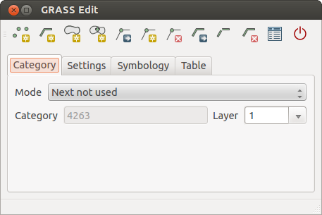
GRASS Digitizing Category Tab

• Mode: The category value that will be applied to new geometry elements.
  • Next not used - Apply next not yet used category value to geometry element.
  • Manual entry - Manually define the category value for the geometry element in the ‘Category’ entry field.
  • No category - Do not apply a category value to the geometry element. This is used, for instance, for area boundaries, because the category values are connected via the centroid.
• Category - The number (ID) that is attached to each digitized geometry element. It is used to connect each geometry element with its attributes.
• Field (layer) - Each geometry element can be connected with several attribute tables using different GRASS geometry layers. The default layer number is 1.

Settings Tab

The Settings tab allows you to set the snapping in screen pixels. The threshold defines at what distance new points or line ends are snapped to existing nodes. This helps to prevent gaps or dangles between boundaries. The default is set to 10 pixels.

Figure GRASS digitizing 3:

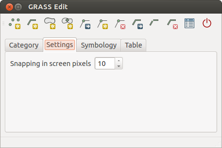
GRASS Digitizing Settings Tab

Symbology Tab

The Symbology tab allows you to view and set symbology and color settings for various geometry types and their topological status (e.g., closed / opened boundary).

Figure GRASS digitizing 4:

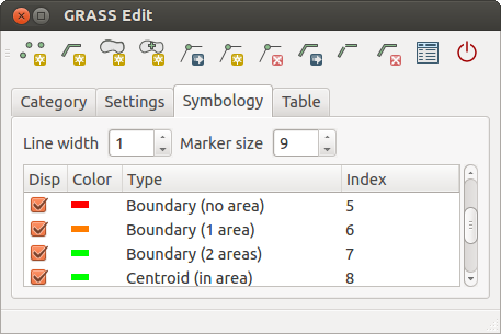
GRASS Digitizing Symbology Tab

Table Tab

The Table tab provides information about the database table for a given ‘layer’. Here, you can add new columns to an existing attribute table, or create a new database table for a new GRASS vector layer (see section Creating a new GRASS vector layer).

Figure GRASS digitizing 5:

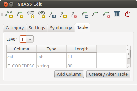
GRASS Digitizing Table Tab

The GRASS region tool¶

The region definition (setting a spatial working window) in GRASS is important for working with raster layers. Vector analysis is by default not limited to any defined region definitions. But all newly created rasters will have the spatial extension and resolution of the currently defined GRASS region, regardless of their original extension and resolution. The current GRASS region is stored in the $LOCATION/$MAPSET/WIND file, and it defines north, south, east and west bounds, number of columns and rows, horizontal and vertical spatial resolution.

It is possible to switch on and off the visualization of the GRASS region in the QGIS canvas using the ^{Display current GRASS region} button.

With the ^{Edit current GRASS region} icon, you can open a dialog to change the current region and the symbology of the GRASS region rectangle in the QGIS canvas. Type in the new region bounds and resolution, and click [OK]. The dialog also allows you to select a new region interactively with your mouse on the QGIS canvas. Therefore, click with the left mouse button in the QGIS canvas, open a rectangle, close it using the left mouse button again and click [OK].

The GRASS module g.region provides a lot more parameters to define an appropriate region extent and resolution for your raster analysis. You can use these parameters with the GRASS Toolbox, described in section The GRASS Toolbox.

The GRASS Toolbox¶

The ^{Open GRASS Tools} box provides GRASS module functionalities to work with data inside a selected GRASS LOCATION and MAPSET. To use the GRASS Toolbox you need to open a LOCATION and MAPSET that you have write permission for (usually granted, if you created the MAPSET). This is necessary, because new raster or vector layers created during analysis need to be written to the currently selected LOCATION and MAPSET.

Figure GRASS Toolbox 1:

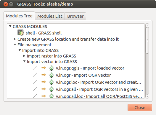
GRASS Toolbox and Module Tree

Working with GRASS modules¶

The GRASS shell inside the GRASS Toolbox provides access to almost all (more than 300) GRASS modules in a command line interface. To offer a more user-friendly working environment, about 200 of the available GRASS modules and functionalities are also provided by graphical dialogs within the GRASS plugin Toolbox.

A complete list of GRASS modules available in the graphical Toolbox in QGIS version 2.8 is available in the GRASS wiki at http://grass.osgeo.org/wiki/GRASS-QGIS_relevant_module_list.

It is also possible to customize the GRASS Toolbox content. This procedure is described in section Customizing the GRASS Toolbox.

As shown in figure_grass_toolbox_1, you can look for the appropriate GRASS module using the thematically grouped Modules Tree or the searchable Modules List tab.

By clicking on a graphical module icon, a new tab will be added to the Toolbox dialog, providing three new sub-tabs: Options, Output and Manual.

Options

The Options tab provides a simplified module dialog where you can usually select a raster or vector layer visualized in the QGIS canvas and enter further module-specific parameters to run the module.

Figure GRASS module 1:

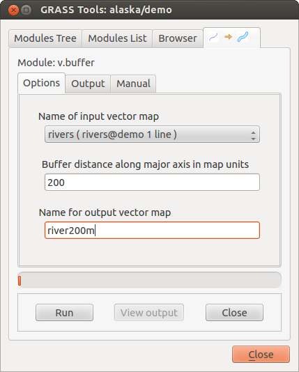
GRASS Toolbox Module Options

The provided module parameters are often not complete to keep the dialog clear. If you want to use further module parameters and flags, you need to start the GRASS shell and run the module in the command line.

A new feature since QGIS 1.8 is the support for a Show Advanced Options button below the simplified module dialog in the Options tab. At the moment, it is only added to the module v.in.ascii as an example of use, but it will probably be part of more or all modules in the GRASS Toolbox in future versions of QGIS. This allows you to use the complete GRASS module options without the need to switch to the GRASS shell.

Output

Figure GRASS module 2:

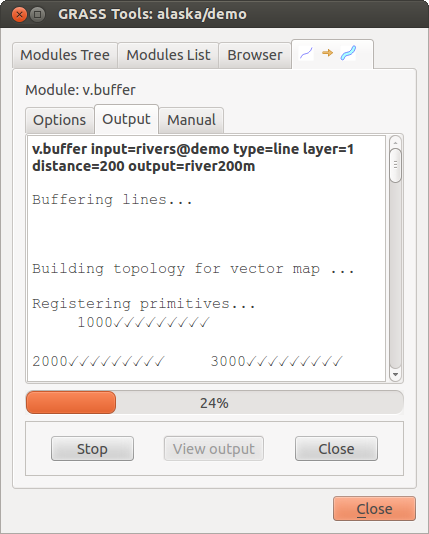
GRASS Toolbox Module Output

The Output tab provides information about the output status of the module. When you click the [Run] button, the module switches to the Output tab and you see information about the analysis process. If all works well, you will finally see a Successfully finished message.

Manual

Figure GRASS module 3:

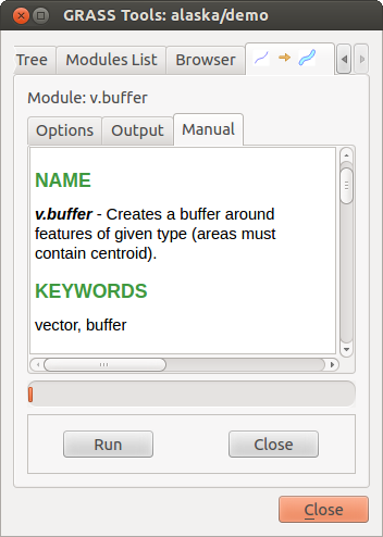
GRASS Toolbox Module Manual

The Manual tab shows the HTML help page of the GRASS module. You can use it to check further module parameters and flags or to get a deeper knowledge about the purpose of the module. At the end of each module manual page, you see further links to the Main Help index, the Thematic index and the Full index. These links provide the same information as the module g.manual.

Tip

Display results immediately

If you want to display your calculation results immediately in your map canvas, you can use the ‘View Output’ button at the bottom of the module tab.

GRASS module examples¶

The following examples will demonstrate the power of some of the GRASS modules.

Creating contour lines¶

The first example creates a vector contour map from an elevation raster (DEM). Here, it is assumed that you have the Alaska LOCATION set up as explained in section Importing data into a GRASS LOCATION.

• First, open the location by clicking the ^{Open mapset} button and choosing the Alaska location.
• Now load the gtopo30 elevation raster by clicking ^{Add GRASS raster layer} and selecting the gtopo30 raster from the demo location.
• Now open the Toolbox with the ^{Open GRASS tools} button.
• In the list of tool categories, double-click Raster ‣ Surface Management ‣ Generate vector contour lines.
• Now a single click on the tool r.contour will open the tool dialog as explained above (see Working with GRASS modules). The gtopo30 raster should appear as the Name of input raster.
• Type into the Increment between Contour levels the value 100. (This will create contour lines at intervals of 100 meters.)
• Type into the Name for output vector map the name ctour_100.
• Click [Run] to start the process. Wait for several moments until the message Successfully finished appears in the output window. Then click [View Output] and [Close].

Since this is a large region, it will take a while to display. After it finishes rendering, you can open the layer properties window to change the line color so that the contours appear clearly over the elevation raster, as in The Vector Properties Dialog.

Next, zoom in to a small, mountainous area in the center of Alaska. Zooming in close, you will notice that the contours have sharp corners. GRASS offers the v.generalize tool to slightly alter vector maps while keeping their overall shape. The tool uses several different algorithms with different purposes. Some of the algorithms (i.e., Douglas Peuker and Vertex Reduction) simplify the line by removing some of the vertices. The resulting vector will load faster. This process is useful when you have a highly detailed vector, but you are creating a very small-scale map, so the detail is unnecessary.

Tip

The simplify tool

Note that the QGIS fTools plugin has a Simplify geometries ‣ tool that works just like the GRASS v.generalize Douglas-Peuker algorithm.

However, the purpose of this example is different. The contour lines created by r.contour have sharp angles that should be smoothed. Among the v.generalize algorithms, there is Chaiken’s, which does just that (also Hermite splines). Be aware that these algorithms can add additional vertices to the vector, causing it to load even more slowly.

• Open the GRASS Toolbox and double-click the categories Vector ‣ Develop map ‣ Generalization, then click on the v.generalize module to open its options window.
• Check that the ‘ctour_100’ vector appears as the Name of input vector.
• From the list of algorithms, choose Chaiken’s. Leave all other options at their default, and scroll down to the last row to enter in the field Name for output vector map ‘ctour_100_smooth’, and click [Run].
• The process takes several moments. Once Successfully finished appears in the output windows, click [View output] and then [Close].
• You may change the color of the vector to display it clearly on the raster background and to contrast with the original contour lines. You will notice that the new contour lines have smoother corners than the original while staying faithful to the original overall shape.

Figure GRASS module 4:

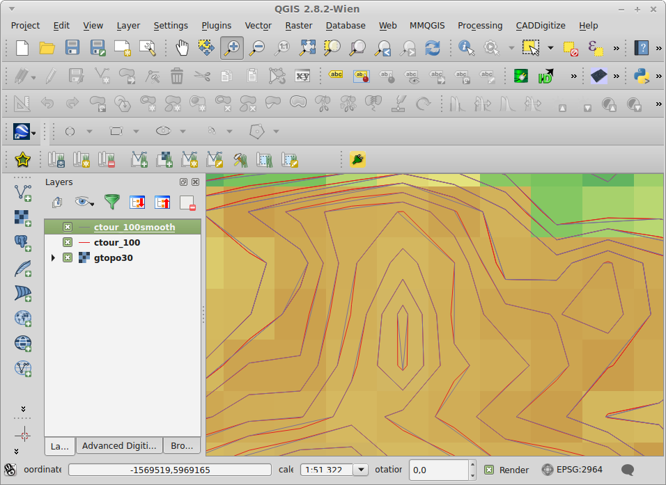
GRASS module v.generalize to smooth a vector map

Tip

Other uses for r.contour

The procedure described above can be used in other equivalent situations. If you have a raster map of precipitation data, for example, then the same method will be used to create a vector map of isohyetal (constant rainfall) lines.

Creating a Hillshade 3-D effect¶

Several methods are used to display elevation layers and give a 3-D effect to maps. The use of contour lines, as shown above, is one popular method often chosen to produce topographic maps. Another way to display a 3-D effect is by hillshading. The hillshade effect is created from a DEM (elevation) raster by first calculating the slope and aspect of each cell, then simulating the sun’s position in the sky and giving a reflectance value to each cell. Thus, you get sun-facing slopes lighted; the slopes facing away from the sun (in shadow) are darkened.

• Begin this example by loading the gtopo30 elevation raster. Start the GRASS Toolbox, and under the Raster category, double-click to open Spatial analysis ‣ Terrain analysis.
• Then click r.shaded.relief to open the module.
• Change the azimuth angle 270 to 315.
• Enter gtopo30_shade for the new hillshade raster, and click [Run].
• When the process completes, add the hillshade raster to the map. You should see it displayed in grayscale.
• To view both the hillshading and the colors of the gtopo30 together, move the hillshade map below the gtopo30 map in the table of contents, then open the Properties window of gtopo30, switch to the Transparency tab and set its transparency level to about 25%.

You should now have the gtopo30 elevation with its colormap and transparency setting displayed above the grayscale hillshade map. In order to see the visual effects of the hillshading, turn off the gtopo30_shade map, then turn it back on.

Using the GRASS shell

The GRASS plugin in QGIS is designed for users who are new to GRASS and not familiar with all the modules and options. As such, some modules in the Toolbox do not show all the options available, and some modules do not appear at all. The GRASS shell (or console) gives the user access to those additional GRASS modules that do not appear in the Toolbox tree, and also to some additional options to the modules that are in the Toolbox with the simplest default parameters. This example demonstrates the use of an additional option in the r.shaded.relief module that was shown above.

Figure GRASS module 5:

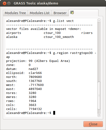
The GRASS shell, r.shaded.relief module

The module r.shaded.relief can take a parameter zmult, which multiplies the elevation values relative to the X-Y coordinate units so that the hillshade effect is even more pronounced.

• Load the gtopo30 elevation raster as above, then start the GRASS Toolbox and click on the GRASS shell. In the shell window, type the command r.shaded.relief map=gtopo30 shade=gtopo30_shade2 azimuth=315 zmult=3 and press [Enter].
• After the process finishes, shift to the Browse tab and double-click on the new gtopo30_shade2 raster to display it in QGIS.
• As explained above, move the shaded relief raster below the gtopo30 raster in the table of contents, then check the transparency of the colored gtopo30 layer. You should see that the 3-D effect stands out more strongly compared with the first shaded relief map.

Figure GRASS module 6:

Displaying shaded relief created with the GRASS module r.shaded.relief

Raster statistics in a vector map¶

The next example shows how a GRASS module can aggregate raster data and add columns of statistics for each polygon in a vector map.

• Again using the Alaska data, refer to Importing data into a GRASS LOCATION to import the trees shapefile from the shapefiles directory into GRASS.
• Now an intermediate step is required: centroids must be added to the imported trees map to make it a complete GRASS area vector (including both boundaries and centroids).
• From the Toolbox, choose Vector ‣ Manage features, and open the module v.centroids.
• Enter as the output vector map ‘forest_areas’ and run the module.
• Now load the forest_areas vector and display the types of forests - deciduous, evergreen, mixed - in different colors: In the layer Properties window, Symbology tab, choose from Legend type ‘Unique value’ and set the Classification field to ‘VEGDESC’. (Refer to the explanation of the symbology tab in Style Menu of the vector section.)
• Next, reopen the GRASS Toolbox and open Vector ‣ Vector update by other maps.
• Click on the v.rast.stats module. Enter gtopo30 and forest_areas.
• Only one additional parameter is needed: Enter column prefix elev, and click [Run]. This is a computationally heavy operation, which will run for a long time (probably up to two hours).
• Finally, open the forest_areas attribute table, and verify that several new columns have been added, including elev_min, elev_max, elev_mean, etc., for each forest polygon.

Working with the GRASS LOCATION browser¶

Another useful feature inside the GRASS Toolbox is the GRASS LOCATION browser. In figure_grass_module_7, you can see the current working LOCATION with its MAPSETs.

In the left browser windows, you can browse through all MAPSETs inside the current LOCATION. The right browser window shows some meta-information for selected raster or vector layers (e.g., resolution, bounding box, data source, connected attribute table for vector data, and a command history).

Figure GRASS module 7:

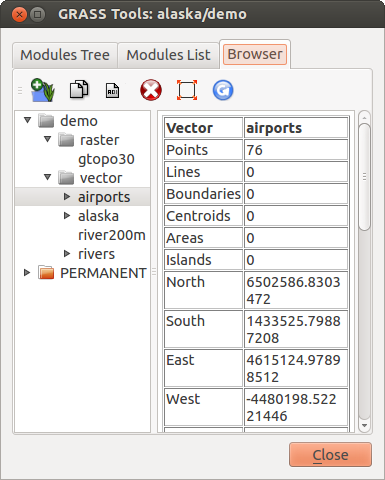
GRASS LOCATION browser

The toolbar inside the Browser tab offers the following tools to manage the selected LOCATION:

• Add selected map to canvas
• Copy selected map
• Rename selected map
• Delete selected map
• Set current region to selected map
• Refresh browser window

The Rename selected map and Delete selected map only work with maps inside your currently selected MAPSET. All other tools also work with raster and vector layers in another MAPSET.

<?xml version="1.0" encoding="UTF-8"?>
<!DOCTYPE qgisgrassmodule SYSTEM "http://mrcc.com/qgisgrassmodule.dtd">

<qgisgrassmodule label="Vector buffer" module="v.buffer">
        <option key="input" typeoption="type" layeroption="layer" />
        <option key="buffer"/>
        <option key="output" />
</qgisgrassmodule>