21. Answer Sheet
21.1. Results For Un’introduzione all’Interfaccia
21.1.1.  Introduzione (Parte 1)
Fate riferimento all’immagine che mostra il layout dell’interfaccia e verificate di ricordare i nomi e le funzioni degli elementi dello schermo.
21.1.2. Introduzione (Parte 2)
Salva come…
Zoom al layer
Inverti selezione
Rendering on/off
Misura linea
21.2. Results For Aggiungere i primi layer
21.2.1. Preparazione
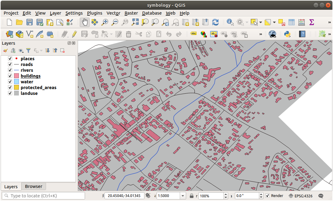
Nell’area principale della finestra di dialogo dovreste vedere molte forme con colori diversi. Ogni forma appartiene a un livello che potete identificare dal suo colore nel pannello di sinistra (i vostri colori potrebbero essere diversi da quelli sotto):

21.2.2. Caricamento dati
La tua mappa dovrebbe avere sette layer:
protected_areas
places
rivers
roads
landuse
buildings (presi da
training_data.gpkg) ewater (presi da
exercise_data/shapefile).
21.3. Results For Simbologia
21.3.1. Colori
Verifica che i colori siano cambiati come ti aspettavi.
È sufficiente scegliere il layer water nella legenda e poi cliccare il pulsante
 Apri il pannello Stile Layerl. Cambia il colore con uno coerente con i layer acqua (water).

Nota
Se desiderate lavorare su un solo livello alla volta e non volete che gli altri livelli vi distraggano, potete nascondere un livello facendo clic sulla casella di controllo accanto al suo nome nell’elenco dei livelli. Se la casella è vuota, il livello è nascosto.
21.3.2. Struttura simbolo
La vostra mappa ora dovrebbe apparire come questa:

Se sei un utente di livello principiante, puoi fermarti qui.
Usate il metodo sopra per cambiare i colori e gli stili per tutti i livelli rimanenti.
Provate a usare colori naturali per gli oggetti. Ad esempio, una strada non dovrebbe essere rossa o blu, ma può essere grigia o nera.
Sentiti libero di sperimentare con differenti impostazioni di Stile riempimento e Stile tratto per i poligoni.

21.3.3.  Layer simbolo
Personalizza il layer buildings come preferisci, ma ricorda che deve essere facile vedere livelli separati sulla mappa.
Ecco un esempio:
21.3.4. Livelli simbolo
Per fare il simbolo richiesto, hai bisogno si tre livelli:

Il simbolo del livello più basso è una linea grigia, larga e uniforme. Sopra di essa c’è una linea gialla stretta e uniforme e infine una linea nera più sottile e uniforme.
Se il tuo simbolo somiglia a quello sopra ma non è il risultato voluto:
Controllo che i livelli del tuo simbolo appaiano come questi:

Ora la tua mappa dovrebbe apparire come questa:

21.3.5.  Livelli simbolo
Regola i livelli del tuo simbolo con questi valori:

Prova con diversi valori per avere risultati differenti.
Apri la tua mappa originale prima di continuare con il prossimo esercizio.
21.4. Simboli contorno
Qui ci sono degli esempi di struttura simbolo:


21.4.1. Geometry generator symbology
Click on the
 button to add another Symbol level.
Move the new symbol at the bottom of the list clicking the
 button.
Choose a good color to fill the water polygons.
Click on Marker of the Geometry generator symbology and change the circle with another shape as your wish.
Try experimenting other options to get more useful results.
21.5. Results For Vector Attribute Data
21.5.1. Exploring Vector Data Attributes
There should be 9 fields in the rivers layer:
Select the layer in the Layers panel.
Right-click and choose Open Attribute Table, or press the
 button on the Attributes Toolbar.
Count the number of columns.
Suggerimento
A quicker approach could be to double-click the rivers layer, open the tab, where you will find a numbered list of the table’s fields.
Information about towns is available in the places layer. Open its attribute table as you did with the rivers layer: there are two features whose place attribute is set to
town: Swellendam and Buffeljagsrivier. You can add comment on other fields from these two records, if you like.The
namefield is the most useful to show as labels. This is because all its values are unique for every object and are very unlikely to contain NULL values. If your data contains some NULL values, do not worry as long as most of your places have names.
21.6. Results For Labels
21.6.1. Label Customization (Part 1)
Your map should now show the marker points and the labels should be offset by 2mm. The style of the markers and labels should allow both to be clearly visible on the map:

21.6.2. Label Customization (Part 2)
One possible solution has this final product:

To arrive at this result:
Use a font size of
10Use an around point placement distance of
1.5 mmUse a marker size of
3.0 mmIn addition, this example uses the Wrap on character option:

Enter a
spacein this field and click Apply to achieve the same effect. In our case, some of the place names are very long, resulting in names with multiple lines which is not very user friendly. You might find this setting to be more appropriate for your map.
21.6.3. Using Data Defined Settings
Still in edit mode, set the
FONT_SIZEvalues to whatever you prefer. The example uses16for towns,14for suburbs,12for localities, and10for hamlets.Remember to save changes and exit edit mode
Return to the Text formatting options for the
placeslayer and selectFONT_SIZEin the Attribute field of the font size data defined override dropdown:
Your results, if using the above values, should be this:

21.7. Results For Classificazione
21.7.1. Refine the Classification
The settings you used might not be the same, but with the values
Classes = 6 and Mode = Natural Breaks
(Jenks) (and using the same colors, of course), the map will look like this:

21.8. Results For Creating a New Vector Dataset
21.8.1. Digitizing
The symbology doesn’t matter, but the results should look more or less like this:

21.8.2. Topology: Add Ring Tool
The exact shape doesn’t matter, but you should be getting a hole in the middle of your feature, like this one:

Undo your edit before continuing with the exercise for the next tool.
21.8.3. Topology: Add Part Tool
First select the Bontebok National Park:

Now add your new part:
Undo your edit before continuing with the exercise for the next tool.
21.8.4. Merge Features
Use the Merge Selected Features tool, making sure to first select both of the polygons you wish to merge.
Use the feature with the OGC_FID of 1 as the source of your attributes (click on its entry in the dialog, then click the Take attributes from selected feature button):
Nota
- If you’re using a different dataset, it is highly likely that your
original polygon’s OGC_FID will not be 1. Just choose the feature which has an OGC_FID.

Nota
Using the Merge Attributes of Selected Features tool will keep the geometries distinct, but give them the same attributes.
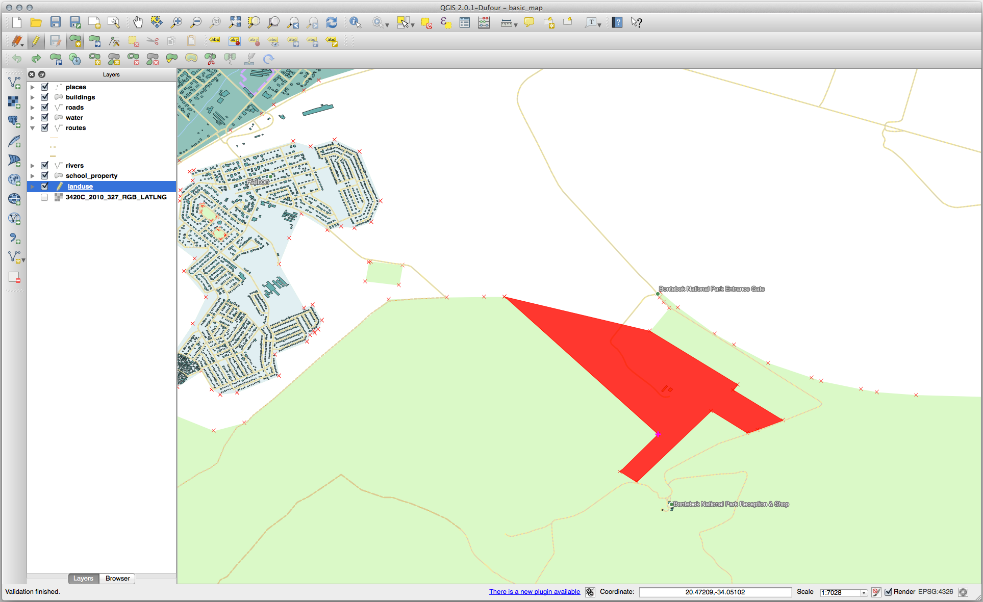
21.8.5. Moduli
Per TYPE, c’è ovviamente un quantità limitata di tipi che una strada può avere, e se controlli la tabella attributi per questo layer, vedrai che sono predefiniti.
Imposta il widget in Mappa Valori e clicca su Carica Dati dal Vettore.
Seleziona roads dalla lista a scomparsa Vettore e highway per le opzioni Valore e Descrizione:

Clicca OK tre volte.
Se usi lo strumento Informazioni su una strada mentre la modalità modifica è attiva, il dialogo che appare dovrebbe essere come questo:
21.9. Results For Vector Analysis
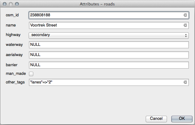
21.9.1. Distance from High Schools
Your buffer dialog should look like this:
The Buffer distance is 1 kilometer.
The Segments to approximate value is set to 20. This is optional, but it’s recommended, because it makes the output buffers look smoother. Compare this:
To this:

The first image shows the buffer with the Segments to approximate value set to 5 and the second shows the value set to 20. In our example, the difference is subtle, but you can see that the buffer’s edges are smoother with the higher value.
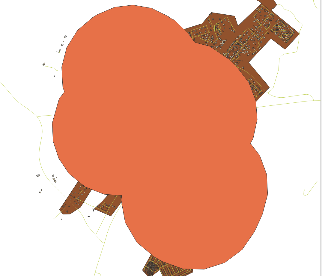
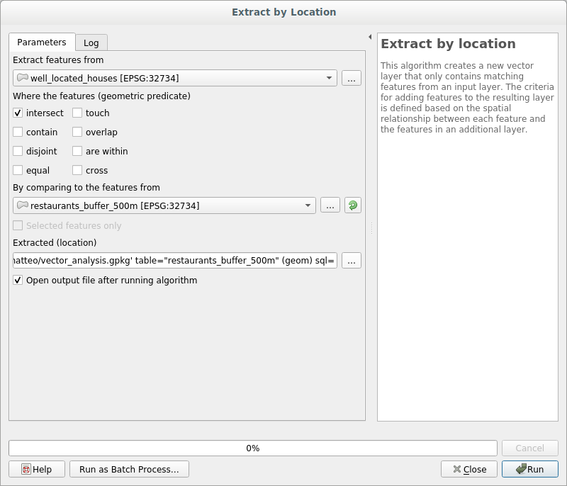
21.9.2. Distance from Restaurants
To create the new houses_restaurants_500m layer, we go through a two step process:
In primo luogo, creare un buffer di 500m intorno ai ristoranti e aggiungere il layer alla mappa:


Successivamente, estrarre gli edifici all’interno di tale buffer area:
La tua mappa dovrebbe mostrare ora solamente gli edifici che si trovano entro 50 metri da una strada, 1 km da una scuola e 500 metri da un ristorante:

21.10. Results For Network Analysis
21.11. Fastest path
Open and fill the dialog as:
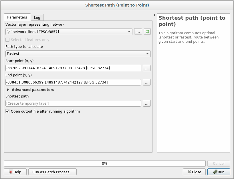
Make sure that the Path type to calculate is Fastest.
Click on Run and close the dialog.
Open now the attribute table of the output layer. The cost field contains the travel time between the two points (as fraction of hours):

21.12. Results For Raster Analysis


21.12.2. Calculate Slope (less than 2 and 5 degrees)
Set your Raster calculator dialog up like this:

For the 5 degree version, replace the
2in the expression and file name with5.
Your results:
2 degrees:
5 degrees:
21.13. Results For Completing the Analysis
21.13.1. Raster to Vector
Open the Query Builder by right-clicking on the all_terrain layer in the Layers panel, and selecting the tab.
Then build the query "suitable" = 1.
Click OK to filter out all the polygons where this condition isn’t met.
When viewed over the original raster, the areas should overlap perfectly:

You can save this layer by right-clicking on the all_terrain layer in the Layers panel and choosing Save As…, then continue as per the instructions.
21.13.2. Inspecting the Results
You may notice that some of the buildings in your new_solution layer have been «sliced» by the Intersect tool. This shows that only part of the building - and therefore only part of the property - lies on suitable terrain. We can therefore sensibly eliminate those buildings from our dataset
21.13.3. Refining the Analysis
At the moment, your analysis should look something like this:

Consider a circular area, continuous for 100 meters in all directions.
If it is greater than 100 meters in radius, then subtracting 100 meters from its size (from all directions) will result in a part of it being left in the middle.

Therefore, you can run an interior buffer of 100 meters on your existing suitable_terrain vector layer. In the output of the buffer function, whatever remains of the original layer will represent areas where there is suitable terrain for 100 meters beyond.
To demonstrate:
Go to to open the Buffer(s) dialog.
Set it up like this:

Use the suitable_terrain layer with 10 segments and a buffer distance of -100. (The distance is automatically in meters because your map is using a projected CRS.)
Save the output in exercise_data/residential_development/ as suitable_terrain_continuous100m.shp.
If necessary, move the new layer above your original suitable_terrain layer.
Your results will look like something like this:

Now use the Select by Location tool ().
Set up like this:

Select features in new_solution that intersect features in suitable_terrain_continuous100m.shp.
This is the result:
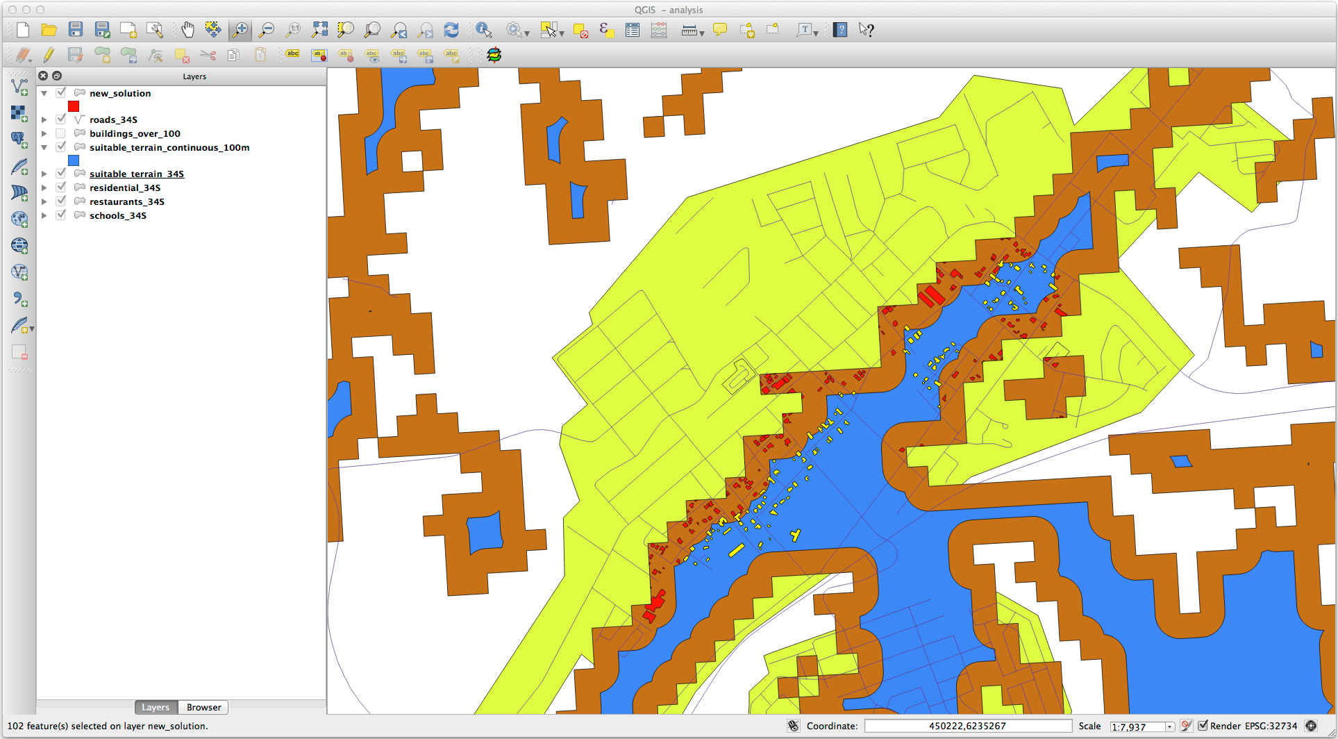
The yellow buildings are selected. Although some of the buildings fall partly outside the new suitable_terrain_continuous100m layer, they lie well within the original suitable_terrain layer and therefore meet all of our requirements.
Save the selection under exercise_data/residential_development/ as final_answer.shp.
21.14. Results For WMS
21.14.1. Adding Another WMS Layer
Your map should look like this (you may need to re-order the layers):

21.14.2. Adding a New WMS Server
Use the same approach as before to add the new server and the appropriate layer as hosted on that server:


If you zoom into the Swellendam area, you’ll notice that this dataset has a low resolution:

Therefore, it’s better not to use this data for the current map. The Blue Marble data is more suitable at global or national scales.
21.14.3. Finding a WMS Server
You may notice that many WMS servers are not always available. Sometimes this is temporary, sometimes it is permanent. An example of a WMS server that worked at the time of writing is the World Mineral Deposits WMS at http://apps1.gdr.nrcan.gc.ca/cgi-bin/worldmin_en-ca_ows. It does not require fees or have access constraints, and it is global. Therefore, it does satisfy the requirements. Keep in mind, however, that this is merely an example. There are many other WMS servers to choose from.
21.15. Results For GRASS Integration
21.15.1. Add Layers to Mapset
You can add layers (both vector and raster) into a GRASS Mapset by drag and drop
them in the Browser (see Follow Along: Load data using the QGIS Browser) or by using the v.in.gdal.qgis
for vector and r.in.gdal.qgis for raster layers.
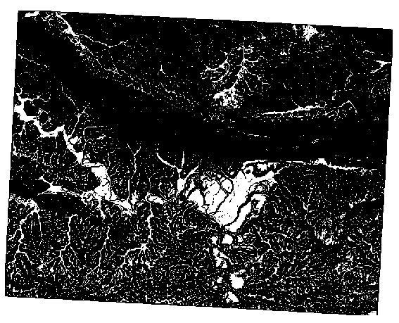
21.15.2. Reclassify raster layer
To discover the maximum value of the raster run the r.info tool: in the console you will see that the maximum value is 1699.
You are now ready to write the rules. Open a text editor and add the following rules:
0 thru 1000 = 1
1000 thru 1400 = 2
1400 thru 1699 = 3
save the file as a my_rules.txt file and close the text editor.
Run the r.reclass tool, choose the g_dem layer and load the file containing the rules you just have saved.
Click on Run and then on View Output. You can change the colors and the final result should look like the following picture:

21.16. Results For Database Concepts
21.16.1. Address Table Properties
For our theoretical address table, we might want to store the following properties:
House Number
Street Name
Suburb Name
City Name
Postcode
Country
When creating the table to represent an address object, we would create columns to represent each of these properties and we would name them with SQL-compliant and possibly shortened names:
house_number
street_name
suburb
city
postcode
country
21.16.2. Normalising the People Table
The major problem with the people table is that there is a single address field which contains a person’s entire address. Thinking about our theoretical address table earlier in this lesson, we know that an address is made up of many different properties. By storing all these properties in one field, we make it much harder to update and query our data. We therefore need to split the address field into the various properties. This would give us a table which has the following structure:
id |     name      | house_no |  street_name   |    city    |   phone_no
 --+---------------+----------+----------------+------------+-----------------
 1 | Tim Sutton    |     3    | Buirski Plein  | Swellendam | 071 123 123
 2 | Horst Duester |     4    | Avenue du Roix | Geneva     | 072 121 122
Nota
In the next section, you will learn about Foreign Key relationships which could be used in this example to further improve our database’s structure.
21.16.3. Further Normalisation of the People Table
Our people table currently looks like this:
id |     name     | house_no | street_id |  phone_no
---+--------------+----------+-----------+-------------
 1 | Horst Duster |        4 |         1 | 072 121 122
The street_id column represents a “one to many” relationship between the people object and the related street object, which is in the streets table.
One way to further normalise the table is to split the name field into first_name and last_name:
id | first_name | last_name  | house_no | street_id |  phone_no
---+------------+------------+----------+-----------+------------
 1 |    Horst   |   Duster   |     4    |     1     | 072 121 122
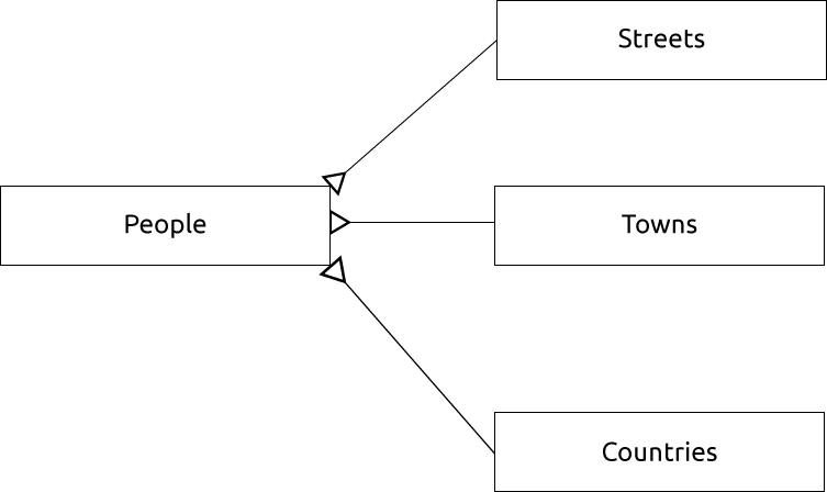
We can also create separate tables for the town or city name and country, linking them to our people table via “one to many” relationships:
id | first_name | last_name | house_no | street_id | town_id | country_id
---+------------+-----------+----------+-----------+---------+------------
 1 |    Horst   |   Duster  |     4    |     1     |    2    |     1
An ER Diagram to represent this would look like this:
21.16.4. Create a People Table
The SQL required to create the correct people table is:
create table people (id serial not null primary key,
                     name varchar(50),
                     house_no int not null,
                     street_id int not null,
                     phone_no varchar null );
The schema for the table (enter \d people) looks like this:
Table "public.people"

Column     |         Type          |                      Modifiers
-----------+-----------------------+-------------------------------------
id         | integer               | not null default
           |                       | nextval('people_id_seq'::regclass)
name       | character varying(50) |
house_no   | integer               | not null
street_id  | integer               | not null
phone_no   | character varying     |
Indexes:
  "people_pkey" PRIMARY KEY, btree (id)
Nota
For illustration purposes, we have purposely omitted the fkey constraint.
21.16.5. The DROP Command
The reason the DROP command would not work in this case is because the people table has a Foreign Key constraint to the streets table. This means that dropping (or deleting) the streets table would leave the people table with references to non-existent streets data.
Nota
It is possible to “force” the streets table to be deleted by using the CASCADE command, but this would also delete the people and any other table which had a relationship to the streets table. Use with caution!
21.16.6. Insert a New Street
The SQL command you should use looks like this (you can replace the street name with a name of your choice):
insert into streets (name) values ('Low Road');
21.16.7. Add a New Person With Foreign Key Relationship
Here is the correct SQL statement:
insert into streets (name) values('Main Road');
insert into people (name,house_no, street_id, phone_no)
  values ('Joe Smith',55,2,'072 882 33 21');
If you look at the streets table again (using a select statement as before), you’ll see that the id for the Main Road entry is 2.
That’s why we could merely enter the number 2 above. Even though we’re not seeing Main Road written out fully in the entry above, the database will be able to associate that with the street_id value of 2.
Nota
If you have already added a new street object, you might find that the new Main Road has an ID of 3 not 2.
21.16.8. Return Street Names
Here is the correct SQL statement you should use:
select count(people.name), streets.name
from people, streets
where people.street_id=streets.id
group by streets.name;
Result:
count |    name
------+-------------
    1 | Low Street
    2 | High street
    1 | Main Road
(3 rows)
Nota
You will notice that we have prefixed field names with table names (e.g. people.name and streets.name). This needs to be done whenever the field name is ambiguous (i.e. not unique across all tables in the database).
21.17. Results For Spatial Queries
21.17.1. The Units Used in Spatial Queries
The units being used by the example query are degrees, because the CRS that the layer is using is WGS 84. This is a Geographic CRS, which means that its units are in degrees. A Projected CRS, like the UTM projections, is in meters.
Remember that when you write a query, you need to know which units the layer’s CRS is in. This will allow you to write a query that will return the results that you expect.
21.17.2. Creating a Spatial Index
CREATE INDEX cities_geo_idx
  ON cities
  USING gist (the_geom);
21.18. Results For Geometry Construction
21.18.1. Creating Linestrings
alter table streets add column the_geom geometry;
alter table streets add constraint streets_geom_point_chk check
     (st_geometrytype(the_geom) = 'ST_LineString'::text OR the_geom IS NULL);
insert into geometry_columns values ('','public','streets','the_geom',2,4326,
     'LINESTRING');
create index streets_geo_idx
  on streets
  using gist
  (the_geom);
21.18.2. Linking Tables
delete from people;
alter table people add column city_id int not null references cities(id);
(capture cities in QGIS)
insert into people (name,house_no, street_id, phone_no, city_id, the_geom)
   values ('Faulty Towers',
           34,
           3,
           '072 812 31 28',
           1,
           'SRID=4326;POINT(33 33)');

insert into people (name,house_no, street_id, phone_no, city_id, the_geom)
   values ('IP Knightly',
           32,
           1,
           '071 812 31 28',
           1,F
           'SRID=4326;POINT(32 -34)');

insert into people (name,house_no, street_id, phone_no, city_id, the_geom)
   values ('Rusty Bedsprings',
           39,
           1,
           '071 822 31 28',
           1,
           'SRID=4326;POINT(34 -34)');
If you’re getting the following error message:
ERROR:  insert or update on table "people" violates foreign key constraint
        "people_city_id_fkey"
DETAIL: Key (city_id)=(1) is not present in table "cities".
then it means that while experimenting with creating polygons for the cities table, you must have deleted some of them and started over. Just check the entries in your cities table and use any id which exists.
21.19. Results For Simple Feature Model
21.19.1. Populating Tables
create table cities (id serial not null primary key,
                     name varchar(50),
                     the_geom geometry not null);
 alter table cities
 add constraint cities_geom_point_chk
 check (st_geometrytype(the_geom) = 'ST_Polygon'::text );
21.19.2. Populate the Geometry_Columns Table
insert into geometry_columns values
      ('','public','cities','the_geom',2,4326,'POLYGON');
21.19.3. Adding Geometry
select people.name,
       streets.name as street_name,
       st_astext(people.the_geom) as geometry
from   streets, people
where  people.street_id=streets.id;
Result:
     name     | street_name |   geometry
--------------+-------------+---------------
 Roger Jones  | High street |
 Sally Norman | High street |
 Jane Smith   | Main Road   |
 Joe Bloggs   | Low Street  |
 Fault Towers | Main Road   | POINT(33 -33)
(5 rows)
As you can see, our constraint allows nulls to be added into the database.