ベクタデータ¶

概要¶

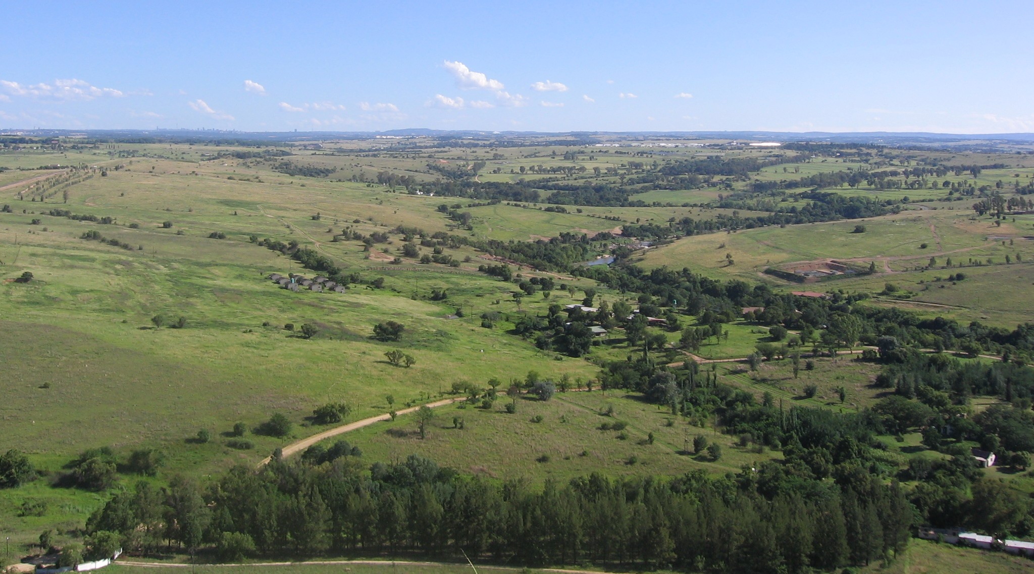
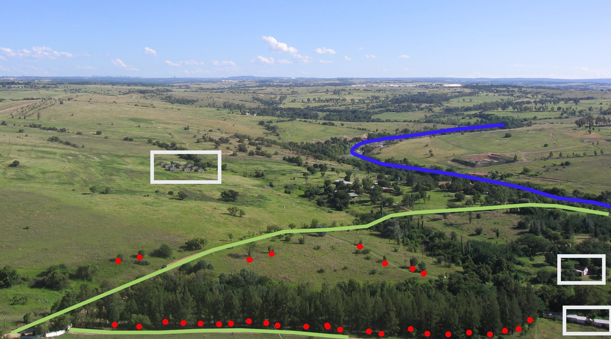
ベクタ は、GISの環境に現実世界の**地物**を表現する1つの手法です。地物は景観に目にすることができものなら何でもです。丘の頂上に立っているところを想像して下さい。見下ろすと家屋、道路、樹木、河川など (figure_landscape_を参照)を見ることができます。これらのもののそれぞれが、GISアプリケーションで表示する時の**地物**です。ベクタ地物は**属性**を持っており、それは地物を**説明する**テキストあるいは数値情報で構成されます。

Figure Landscape 1:

道路、家屋、樹木などの主要な地物が見える景観を見渡す。

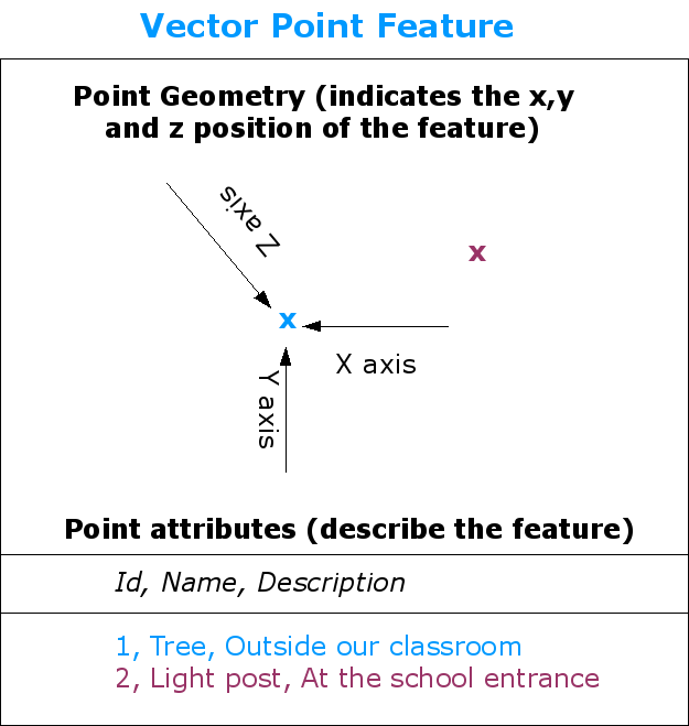
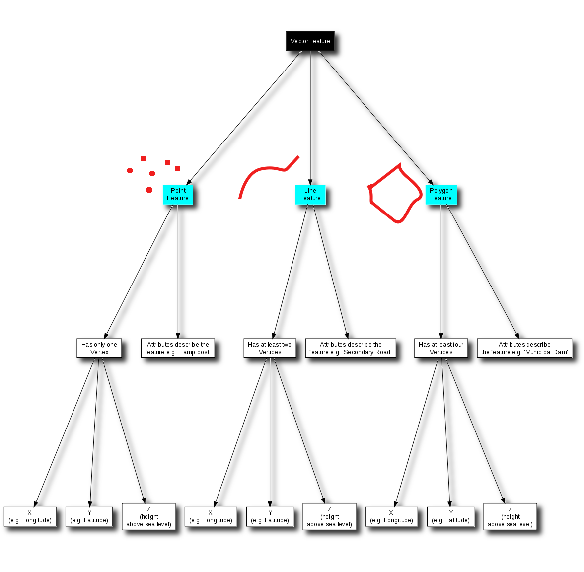
ベクタ形式の地物は、ジオメトリ**を用いて形状を表します。ジオメトリは1つまたはそれ以上の相互につながった**頂点**で作られます。頂点は空間における位置を**X, Y そして必要に応じて **z**軸を用いて表します。``Z``軸がある頂点を持ったジオメトリは、それぞれの頂点の高さあるいは深さ（両方ではない）を表すため、しばしば**2.5D**と呼ばれます。

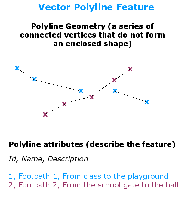
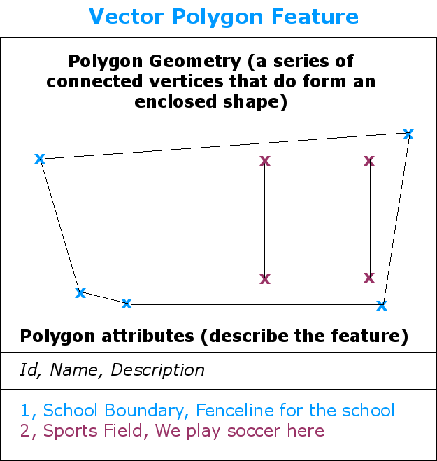
When a feature’s geometry consists of only a single vertex, it is referred to as a point feature (see illustration figure_geometry_point). Where the geometry consists of two or more vertices and the first and last vertex are not equal, a polyline feature is formed (see illustration figure_geometry_polyline). Where three or more vertices are present, and the last vertex is equal to the first, an enclosed polygon feature is formed (see illustration figure_geometry_polygon).

Figure Vector Geometries 1:

ポイント地物は、そのX, Y と必要に応じて Z 座標で表現されます。ポイント属性は、そのポイントが例えば樹木あるいは街灯であるかどうかを表します。

Figure Vector Geometries 2:

ポリラインは一連の結合された頂点です。それぞれの頂点は X, Y (そして必要に応じて Z)座標を持ちます。属性はポリラインを表します。

Figure Vector Geometries 3:

ポリゴンはポリラインのように、一連の頂点です。しかし1つのポリゴンにおいて、最初と最後の頂点は常に同じ位置にあります。

先にご覧いただいた景観写真を見直してみると、GISが表している異なるタイプの地物を見ることができるはずです。 (see illustration figure_geometry_landscape)

Figure Landscape 2:

GISで表現する際の景観地物。河川(青)と道路(緑)はラインで、樹木はポイント(赤)で、家屋はポリゴン(白)で表される。

ポイント地物の詳細¶

ポイント地物について説明する際に最初に認識する必要があることは、GISでポイントとして表示するものは、考え方にもよるが、しばしば縮尺に依存します。例として都市を見てみましょう。もし小縮尺の地図(広いエリアをカバーする)を持っている場合、都市をポイント地物として表すのが適しています。しかし、大縮尺へと地図をズームさせるにつれて、ポリゴンで都市の境界を表示する方がふさわしくなります。

ポイントで地物を表示することを選択する場合、スケール(どれだけその地物から離れているか)、利便さ(ポリゴン地物よりもポイント地物を作成する方が時間と労力が少なくなります)、地物のタイプ(電話のポールのようなポリゴンで格納することが単に意味が無いもの)が大方左右します

As we show in illustration figure_geometry_point, a point feature has an X, Y and optionally, Z value. The X and Y values will depend on the Coordinate Reference System (CRS) being used. We are going to go into more detail about Coordinate Reference Systems in a later tutorial. For now let’s simply say that a CRS is a way to accurately describe where a particular place is on the earth’s surface. One of the most common reference systems is Longitude and Latitude. Lines of Longitude run from the North Pole to the South Pole. Lines of Latitude run from the East to West. You can describe precisely where you are at any place on the earth by giving someone your Longitude (X) and Latitude (Y). If you make a similar measurement for a tree or a telephone pole and marked it on a map, you will have created a point feature.

我々は地球は平らではない知っているので、点の地物にはZ値を追加すると便利です。これは、あなたにどのように海抜が高いかについて説明します。

ポリライン地物の詳細¶

Where a point feature is a single vertex, a polyline has two or more vertices. The polyline is a continuous path drawn through each vertex, as shown in figure_geometry_polyline. When two vertices are joined, a line is created. When more than two are joined, they form a ‘line of lines’, or polyline.

A polyline is used to show the geometry of linear features such as roads, rivers, contours, footpaths, flight paths and so on. Sometimes we have special rules for polylines in addition to their basic geometry. For example contour lines may touch (e.g. at a cliff face) but should never cross over each other. Similarly, polylines used to store a road network should be connected at intersections. In some GIS applications you can set these special rules for a feature type (e.g. roads) and the GIS will ensure that these polylines always comply to these rules.

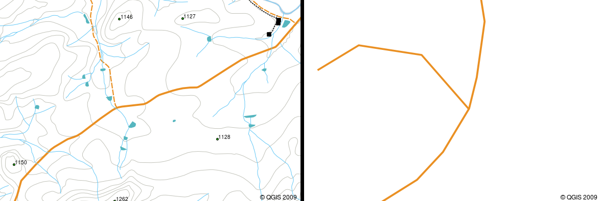
If a curved polyline has very large distances between vertices, it may appear angular or jagged, depending on the scale at which it is viewed (see figure_polyline_jagged). Because of this it is important that polylines are digitised (captured into the computer) with distances between vertices that are small enough for the scale at which you want to use the data.

Figure Polyline 1:

小さいスケール（1：20 000左側に）で見てポリラインが滑らかに湾曲し表示されることがあります。大スケール（1:500 より右に）にズームするとポリラインはとても角ばって見えるかもしれません。

The attributes of a polyline decribe its properties or characteristics. For example a road polyline may have attributes that describe whether it is surfaced with gravel or tar, how many lanes it has, whether it is a one way street, and so on. The GIS can use these attributes to symbolise the polyline feature with a suitable colour or line style.

ポリゴン地物の詳細¶

Polygon features are enclosed areas like dams, islands, country boundaries and so on. Like polyline features, polygons are created from a series of vertices that are connected with a continuous line. However because a polygon always describes an enclosed area, the first and last vertices should always be at the same place! Polygons often have shared geometry –– boundaries that are in common with a neighbouring polygon. Many GIS applications have the capability to ensure that the boundaries of neighbouring polygons exactly coincide. We will explore this in the トポロジ topic later in this tutorial.

ポイントとポリラインと同様に、ポリゴンは**属性**を持っています。属性は、ポリゴンごとに記述します。例えば、ダムは深さと水質の属性を持っている可能性があります。

レイヤ内のベクタデータ¶

Now that we have described what vector data is, let’s look at how vector data is managed and used in a GIS environment. Most GIS applications group vector features into layers. Features in a layer have the the same geometry type (e.g. they will all be points) and the same kinds of attributes (e.g. information about what species a tree is for a trees layer). For example if you have recorded the positions of all the footpaths in your school, they will usually be stored together on the computer hard disk and shown in the GIS as a single layer. This is convenient because it allows you to hide or show all of the features for that layer in your GIS application with a single mouse click.

ベクタデータの編集¶

The GIS application will allow you to create and modify the geometry data in a layer –– a process called digitising –– which we will look at more closely in a later tutorial. If a layer contains polygons (e.g. farm dams), the GIS application will only allow you to create new polygons in that layer. Similarly if you want to change the shape of a feature, the application will only allow you to do it if the changed shape is correct. For example it won’t allow you to edit a line in such a way that it has only one vertex –– remember in our discussion of lines above that all lines must have at least two vertices.

Creating and editing vector data is an important function of a GIS since it is one of the main ways in which you can create personal data for things you are interested in. Say for example you are monitoring pollution in a river. You could use the GIS to digitise all outfalls for storm water drains (as point features). You could also digitise the river itself (as a polyline feature). Finally you could take readings of pH levels along the course of the river and digitise the places where you made these readings (as a point layer).

あなた自身のデータを作成するだけでなく、たくさんの入手および利用可能なフリーのベクタデータがあります。たとえば、Chief Directorate: Surveys and Mappingから 1:50 000 のマップシートで表示されるベクタデータを入手できます。

縮尺とベクタデータ¶

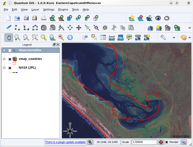
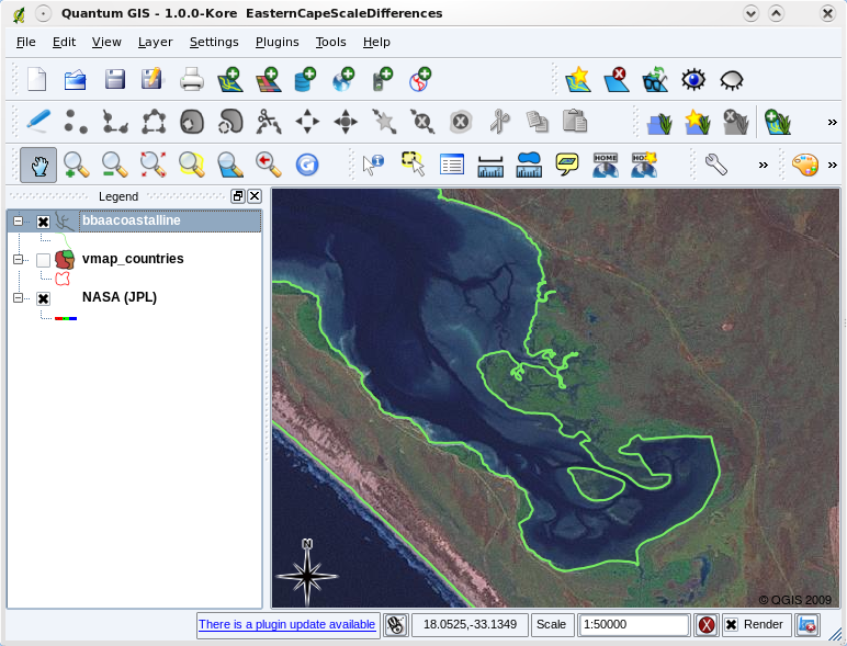
Map scale is an important issue to consider when working with vector data in a GIS. When data is captured, it is usually digitised from existing maps, or by taking information from surveyor records and global positioning system devices. Maps have different scales, so if you import vector data from a map into a GIS environment (for example by digitising paper maps), the digital vector data will have the same scale issues as the original map. This effect can be seen in illustrations figure_vector_small_scale and figure_vector_large_scale. Many issues can arise from making a poor choice of map scale. For example using the vector data in illustration figure_vector_small_scale to plan a wetland conservation area could result in important parts of the wetland being left out of the reserve! On the other hand if you are trying to create a regional map, using data captured at 1:1000 000 might be just fine and will save you a lot of time and effort capturing the data.

Figure Vector Scale 1:

小スケール（1:1000000）マップからデジタル化されたベクタデータ（赤線）。

Figure Vector Scale 2:

大スケール（1：50000）のマップからデジタル化されたベクタデータ（緑色の線）。

シンボロジー¶

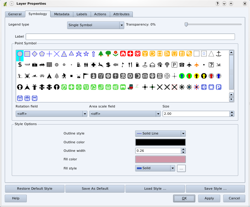
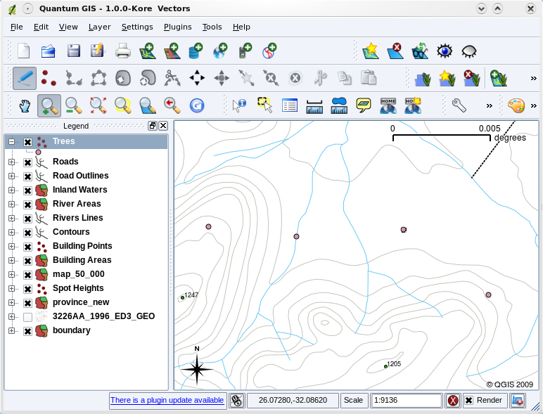
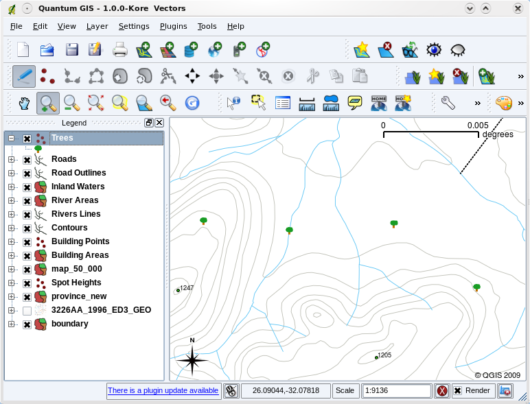
When you add vector layers to the map view in a GIS application, they will be drawn with random colours and basic symbols. One of the great advantages of using a GIS is that you can create personalised maps very easily. The GIS program will let you choose colours to suite the feature type (e.g. you can tell it to draw a water bodies vector layer in blue). The GIS will also let you adjust the symbol used. So if you have a trees point layer, you can show each tree position with a small picture of a tree, rather than the basic circle marker that the GIS uses when you first load the layer (see illustrations figure_vector_symbology, figure_generic_symbology and figure_custom_symbology).

Figure Vector Symbology 1:

GISでは、レイヤ内のフィーチャを描画する方法を調整する（上記のような）パネルを使用することができます。

Figure Vector Symbology 2:

レイヤ（例えば上にある木のレイヤ）が初めてロードされると、GISアプリケーションは一般的なシンボルを与えます。

Figure Vector Symbology 3:

調整を行った後、木を表現するようにポイントが見えた方がはるかに無難です。

Symbology is a powerful feature, making maps come to life and the data in your GIS easier to understand. In the topic that follows (ベクタ属性データ) we will explore more deeply how symbology can help the user to understand vector data.

我々は、GISにおいてベクタデータで何ができる？¶

At the simplest level we can use vector data in a GIS Application in much the same way you would use a normal topographic map. The real power of GIS starts to show itself when you start to ask questions like ‘which houses are within the 100 year flood level of a river?’; ‘where is the best place to put a hospital so that it is easily accessible to as many people as possible?’; ‘which learners live in a particular suburb?’. A GIS is a great tool for answering these types of questions with the help of vector data. Generally we refer to the process of answering these types of questions as spatial analysis. In later topics of this tutorial we will look at spatial analysis in more detail.

ベクタデータの一般的な問題¶

Working with vector data does have some problems. We already mentioned the issues that can arise with vectors captured at different scales. Vector data also needs a lot of work and maintenance to ensure that it is accurate and reliable. Inaccurate vector data can occur when the instruments used to capture the data are not properly set up, when the people capturing the data aren’t being careful, when time or money don’t allow for enough detail in the collection process, and so on.

If you have poor quality vector data, you can often detect this when viewing the data in a GIS. For example slivers can occur when the edges of two polygon areas don’t meet properly (see figure_vector_slivers).

Figure Vector Issues 1:

Slivers occur when the vertices of two polygons do not match up on their borders. At a small scale (e.g. 1 on left) you may not be able to see these errors. At a large scale they are visible as thin strips between two polygons (2 on right).

Overshoots can occur when a line feature such as a road does not meet another road exactly at an intersection. Undershoots can occur when a line feature (e.g. a river) does not exactly meet another feature to which it should be connected. Figure figure_vector_overshoots demonstrates what undershoots and overshoots look like.

Figure Vector Issues 2:

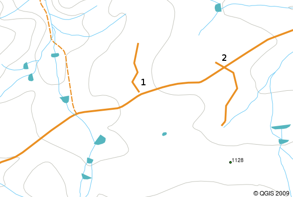
Undershoots (1) occur when digitised vector lines that should connect to each other don’t quite touch. Overshoots (2) happen if a line ends beyond the line it should connect to.

Because of these types of errors, it is very important to digitise data carefully and accurately. In the upcoming topic on topology, we will examine some of these types of errors in more detail.

わかりましたか?¶

ここでは以下のことを学びました:

• GISにおいて、**ベクタデータ**は現実世界を代表する**地物**を表現するために利用されます。

• ベクタの地物は**点**、 **線**または**ポリゴン**の**ジオメトリ**タイプを持つことができます。

• 各ベクタの地物は、**属性データ**を持ち、それを記述します。

• 地物のジオメトリ（幾何形状）は **頂点**の観点で記述されます。

• ポイントジオメトリは、**1つの頂点**（X、Yおよび任意でZ）で構成されています。

• ポリラインジオメトリは ラインをつないで形成する**２つ以上の**頂点で構成されています。

• ポリゴンジオメトリは閉じたエリアを形成する**少なくとも４つの頂点**で構成されています。最初と最後の頂点は常に同じ位置です。

• 使用するジオメトリタイプの選択は、スケール、利便性とGISにおいてデータで何をやりたいかに依存します。

• ほとんどのGISアプリケーションでは、単一のレイヤで複数のジオメトリタイプを混在させることはできません。

• デジタイジングは、GISアプリケーションで描画することにより、デジタルベクタデータを作成するプロセスです。

• Vector data can have quality issues such as undershoots, overshoots and slivers which you need to be aware of.

• GISアプリケーションではベクタデータを**空間分析**に利用できます。例えば、学校に近い病院を見つけるなどです。

Figure figure_vector_summary_で、GISのベクタデータのコンセプトをまとめました。

Figure Vector Summary 1:

この図は、GISアプリケーションがベクタデータを扱う方法を示しています。

やってみよう¶

ここでは人に教える際のアイデアいくつか述べていきます:

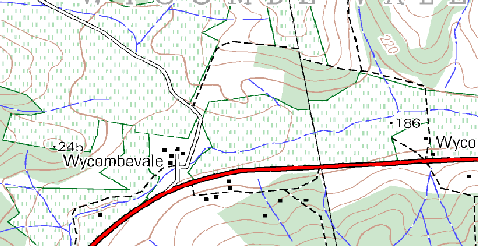
• Using a copy of a toposheet map for your local area (like the one shown in figure_sample_map), see if your learners can identify examples of the different types of vector data by highlighting them on the map.
• Think of how you would create vector features in a GIS to represent real world features on your school grounds. Create a table of different features in and around your school and then task your learners to decide whether they would be best represented in the GIS as a point, line or polygon. See table_vector_1 for an example.

Figure Sample Map 1:

このマップ上の2点の地物と1つのポリゴンを識別することができますか？

Table Vector 1: Create a table like this (leaving the geometry type column empty) and ask your learners to decide on suitable geometry types.

考えてみよう¶

If you don’t have a computer available, you can use a toposheet and transparency sheets to show your learners about vector data.

より詳しく知りたい場合は¶

The QGIS User Guide also has more detailed information on working with vector data in QGIS.

次は?¶

In the section that follows we will take a closer look at attribute data to see how it can be used to describe vector features.